DoublePendulum: A WPF 3D Simulation to Inspect the Dynamics of a Double Pendulum

• Download demo - 166.4 KB
• Download source - 183.8 KB

Introduction

A double pendulum is a simple physical system that exhibits rich dynamic behavior with a strong sensitivity to initial conditions. At low energies the motion is periodic and quasiperiodic and gets more and more chaotic with higher energies. At very high energies the chaos disappears again.

The DoublePendulum application lets you specify initial conditions graphically in two different ways and shows the resulting motion in a 2D and 3D view of the pendulum. To study the long term behavior, a Poincaré map is used, which shows the phase state of the system at certain points in time.

Background

The motion of a double pendulum can be well described by means of an area of physics called Classical Mechanics. The equations of motion can be solved by using the Langrange formalism. I am not going to explain this formalism here, but you should have an understanding of the so called phase space of a mechanical system, so let's go one step back, and have a look at a simple pendulum.

A Simple (Planar) Pendulum

When we displace a simple planar pendulum from its resting position and release it, it will swing back and forth in an always periodic way. If there is no friction, it will move in the same way until the end of time. And the pendulums we are talking about are pure mathematical systems without any friction. Since the motion is planar, we can use a 2D coordinate system to show the position of the pendulum at a certain time as in this picture from Wikipedia:

In the end the motion can be described with a single scalar equation for the angle Θ. Both x and y can be calculated from Θ because the length of the rod is constant over time.

Degrees Of Freedom And The Phase Space

A degree of freedom is an independent physical parameter in the formal description of the state of a physical system. In our case the angle Θ is such an independent parameter. It turns out that we only need a second parameter to describe the state of a simple pendulum completely: the angular velocity ω. If we know Θ and ω at a certain time, we can calculate the motion for all times.

The phase space of a dynamical system is a space in which all possible states of a system are represented, with each possible state corresponding to one unique point in the phase space. Over time a dynamic system moves from one state to another, which leads to a phase space trajectory.

In our case this trajectory looks very simple. If the angle Θ is at its maximum, the angular velocity ω is 0. If the pendulum moves down to its equilibrium position, the velocity increases and reaches its maximum at Θ = 0. Now when the pendulum is moving up to its maximum angle at the opposite side (Θ < 0), its velocity decreases and gets 0 at the maximum (Θ = -Θmax). Now the pendulum is moving down again and the velocity increases, but with a different sign now. The resulting trajectory in phase space is something circular as in this picture:

Instead of the angular velocity ω, the corresponding angular momentum L can also be used to describe the state of a rotating system. In our case the angular momentum is simply r²*m*ω, with r being the length of the rod and m being the mass of the bob (which are both set to 1 in the simulation).

Constant Total Energy And The Loss Of Freedom

As being said before, angle and angular velocity (or momentum) are the two degrees of freedom for the simple pendulum. But if there is no friction in the motion, the total energy of the pendulum will not change over time. And since the total energy is a function of angle and velocity, we can calculate one these properties when knowing the other and the total energy. That means that a frictionless pendulum loses one of its degrees of freedom.

That also means that the trajectory in phase space is a one-dimensional subset of the two-dimensional space. In our case a circle in a plane.

A Planar Double Pendulum

If we attach a second pendulum to the end of a simple pendulum, it's what we call a double pendulum:

The independent physical parameters of this system are again the angle and angular momentum of the first mass, but since the second mass can move on its own, its angle and angular momentum are also independent parameters. So the double pendulum has four degrees of freedom.

The total energy is now a function of four parameters, and if there is no friction, this energy again will be constant. So if we know the total energy, we can calculate one of the four parameters if we know the other three. So again the system loses one degree of freedom and the phase space trajectory is a three-dimensional subset of the four-dimensional phase space.

The Poincaré Map

The French mathematician and physicist Jules Henri Poincaré had a great idea which helps us to visualize the long term behavior of our system. The trick is to cut out a section of the multi-dimensional phase space by setting one of the independent parameters to a certain value and check when the system crosses this so called Poincaré section.

If, for example, the phase space is three-dimensional with parameters x, y and z, the trajectory of that system would be a path in a 3D world, let's say the room we are sitting in right now. Our system could be a particle that is flying through that room. If we now mount a permeable plane in the middle of our room, the particle will cross this plane from time to time. Whenever this happens, we add a mark on the plane at the crossing point.

If the movement of our particle is non-periodic (or chaotic), it will cross the plane at random points. And even if it crosses the plane at a point that already had been marked, it might fly into a completely different direction than it did before. If we wait long enough, our plane will be covered with markers all over.

But what if the movement is periodic? The simplest case would be a particle that is swinging forth and back. If we mounted our plane somewhere in the middle of that movement, the particle will cross that plane at always the same point. So there will be a single mark on the plane.

If the movement is a bit more complex, but still periodic, e.g. if the particle is flying in a circle, there will be two marks on the plane (presuming we mounted the plane at the right place). And if we now think of an even more complex (but still periodic) movement, there will be a finite set of markers on the crossing plane in the end. That's because at some point in time, the movement of our particle repeats itself.

So the Poincaré map of a system gives us an immediate impression of the dynamic behavior: a simple periodic behavior will be represented by a few or even a single point in the map, whereas complex periodic behavior is represented by many but a finite number of points. Chaotic behavior reveals itself by an infinite number of points which are randomly spread around the map.

The Poincaré Condition For The Double Pendulum

In the example before, where the Poincaré map is a 2D plane in a 3D phase space, it is important to choose the right location and orientation for the plane. If we put it somewhere, where the system never crosses that plane, it wouldn't help that much. So we have to identify which one of the four parameters of our double pendulum (Θ1, L1, Θ2 or L2) is a good candidate for building the Poincaré section. I am going to use the angular momentums L1 and L2 instead of angular velocities ω1 and ω2.

If the pendulum is moving at low energy, both Θ1 and Θ2 will take values near the equilibrium value of Θ = 0. And also for higher energies, where the masses start to flip over, it will happen very often, that one of these angles is 0. So let's go with Θ2 = 0. With this condition we can reduce the 4D phase space to a 3D section.

Again, since the total energy is constant, we can calculate one of the remaining 3 parameters, if we know 2 of them. So if we know the total energy E0 and Θ1 and the corresponding L1, we should be able to calculate L2 under the condition that Θ2 is 0. It turns out that there will be two solutions to this problem in most cases: one means that the lower pendulum is swinging from the left to the right of its lowest position, while it could also swing from the right to the left.

To come to a unique solution we just specify that we only accept states where the lower pendulum is swinging from the left to the right, which means that its angular velocity is greater than zero. So the complete Poincaré condition is Θ2 = 0 and ω2 > 0.

Based on the above, we can use a 2D diagram to represent the full state of our 4D system under the Poincaré condition. The diagram shows Θ1 on its x axis and L1 on the y axis. If now E0 is known, a point in the diagram leads to L2, because we also know that Θ2 = 0 and ω2 > 0 for all points in that map.

Enough Theory!

Let's start the application and have a look around. The main window has three views:

• A 3D view of the pendulum showing the actual motion (created with the WFTools3D library)
• A 2D view of the pendulum to set up initial values and showing the actual motion
• A Poincare map showing (Θ1, L1) values of the latest simulations which can also be used to start a new simulation

The 2D view allows you to set up initial values for Θ1 and Θ2 as well as for ω1 and ω2. You can simply drag one of the masses with the left mouse button. If you do so, the 3D view will be updated accordingly. You will also notice that the total energy E0 changes. The energy is not measured in SI units, but in units of m*g*l (m = mass of a bob, l = length of rod), which makes it easy to interpret the values.

If the total energy is 0, both pendulums are at their lowest position and have no velocity. A value of 1 could mean, that one of the masses is raised by one length unit. The following picture shows the double pendulum at different energies:

To get started, let's choose initial values for Θ1 and Θ2 so that the total energy is about 0.01. Move the first mass to its lowest position and the second mass just a little bit to the left like this:

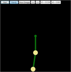
If you now start the simulation by clicking the Start button, you can see the motion in both the 2D and the 3D view. Each time, when the system passes the Poincaré section, i.e. when the lower mass swings from the left to the right of its lowest position, the bob in the 2D view will flash in red and a new point is added to the Poincaré map.

In fact you will notice that two points are added to the Poincaré diagram. That's because the mirror symmetry of our system allows us to do so. If the point (Θ1, L1) belongs to a trajectory in phase space, then the point (-Θ1, L1) belongs to a trajectory which is closely related. It might not be the same trajectory, but to fill up the Poincaré map more quickly, I have chosen to add that second point also.

After a short while the Poincaré diagram will look like this:

The motion is obviously not periodic (which we can also see in the 2D and 3D view), but it is also not chaotic, because the points are not randomly spread around the map but seem to form a certain shape. If we wait a bit longer, the map looks like this:

We can now speed up the simulation by clicking the ">>" button. After a minute or so there should be lots of points with (nearly) no empty space between them:

Even if we now wait longer, that picture will not change. For sure new points will be added, but they will be so close to an already existing point, that there is no visual difference. If a new point would exactly match an existing point, the motion would repeat itself from this point on. That would mean a periodic motion. But in this case we can assume that new points will be added somewhere in-between two existing points and the points form a curve in the 2D space. This behavior is called quasiperiodic because at some point in time two points will be so close to each other that we cannot see a difference in the motion from then on.

Adding Another Trajectory

Stop the simulation by clicking the Stop button. We will now add another trajectory to the Poincaré map. To do so, just do a right mouse button click somewhere above the upper part of the existing curve, e.g. at a position which is shown here:

If you release the mouse button, the new simulation will directly start. The points which are now added to the map will form a curve nearly just like the ones before with just a small offset. While the simulation is running you can click one of the color buttons to change the color for the points of this simulation.

The fact that choosing initial system parameters which are close to another set of parameters lead to nearly the same behavior, shows the non-chaotic behavior of our system. Chaos means that a slight change in the initial setup leads to a complete different behavior.

Adding More Trajectories

You can stop the simulation by doing a right click in the Poincaré diagram. Add another simulation again slightly above the last one and change its color to something different. The result might look like this:

This time the resulting curve seems to form a closed shape (in cyan). That's an interesting thing, because it would mean that whenever we choose an initial point inside of this shape, all following points would also lie within this shape. Otherwise, if there would be a crossing point, the system would behave as before, meaning that all following points would lie on the border formed by the previous trajectory. So let's check this by stopping the current simulation and adding a new initial point inside of the shape. On my side the result looks like this:

And indeed the new motion forms a closed shape within the previous one. Obviously there is something special with the motion in the middle of that shape. So stop the simulation and start a new one somewhere in the middle with the right mouse button. Here's my result:

What seems to be a single red dot in the middle of the concentric curves are in fact many points very close to each other. And that means that the double pendulum is now moving in a periodic way. And if you look at the 2D or 3D view, you will notice that indeed both pendulums are swinging forth and back in the same way. They are swinging nearly exactly inphase.

By the way, if you are not happy with your current simulation and want to get rid of the points, just stop the simulation and do a ctrl-right click. We can now zoom into the Poincaré diagram with the left mouse button. Just drag a rectangle around the center point like this:

That shows us, that the motion is not strictly periodic, but we could go on adding new simulations by clicking into the center of the shape and zoom into the result again. In this way we would be able to come as close as we want to the singular periodic motion.

But for now let's zoom out again by dragging the mouse to the top left corner. If you move the mouse just a little bit, it will take you one zoom step back, while a large movement will take you to the whole picture again.

Now let's have a look at the lower part of the map. Add a new simulation just below the upper curve of the first simulation. It might look like this:

Once again the points in the Poincaré diagram form a closed shape (in blue), and we already know that at the center of this shape there will be another periodic motion. You will find it easily by adding a few more simulations:

Although the red dot in the middle of the lower concentric curves might show up as yet another curve if we zoom in, it shows us that the pendulum is at least very near to a periodic orbit. Look at the 2D and 3D view and you'll see that both pendulums are moving in nearly exact antiphase. If the upper mass moves to the right, the lower mass moves to the left and vice versa.

Summary For Low Energy Motions

When moving at low energy, there are only two periodic orbits: an inphase and an antiphase oscillation. These two motions are of very high order: their representation in the Poincaré map is made up of a single point only. All other motions are quasiperiodic and kind of satellites of one of the periodic orbits.

Furthermore it is worth to mention again that whenever the points of a long running simulation form a closed shape, we will find a periodic motion in the middle of that shape.

The Double Pendulum At Higher Energies

The following sections describe the behavior of the double pendulum if we raise the energy step by step. It turns out that in the begin new periodic oscillations with decreasing order will appear. Decreasing order means that the number of Poincaré points for that motions will increase. So the motion is still periodic, but more complex. All in all the phase space is dominated by quasiperiodic motions.

If the total energy reaches about 0.8, something new happens: one of the curves which show quasiperiodic motion starts to blur out. Instead of being a crisp line it shows up as a band and the bandwidth gets larger with increasing energy. Very soon the band will occupy a large amount of the phase space and this is where chaos comes in.

At the energy of 4.5 all periodic and quasiperiodic oscillations have disappeared and every motion is chaotic. But soon there will be new periodic motions starting with an energy of 5. The pendulum now has enough energy for rotations and for most of the periodic motions the two pendulums will rotate in either the same direction or in opposite directions.

For very high energies (> 1000) most of the periodic motions again will disappear and quasiperiodic motions dominate the scene. In the end, there is no chaos anymore and all motions are quasiperiodic with a single periodic rotation. The same would happen if there was no gravity.

E0 = 0.1

Just as before there are two periodic oscillations (inphase and antiphase) and all other motions are quasiperiodic.

E0 = 0.2

A new periodic motion shows up in the inphase region which is represented by the three closed curves in green.

E0 = 0.25

Another new periodic motion shows up in the antiphase region which is represented by the four closed curves in magenta.

E0 = 0.3

The area of influence of the two new periodic motions gets larger. While the upper curves are moving towards the inphase state, the lower ones are moving away from the antiphase state.

E0 = 0.4

The areas of influence are getting larger again. These areas can be seen as attractors for the periodic motion in the middle. If the pendulum starts at a position within an attractor, it will wobble around the corresponding periodic motion. Note that the magenta attractor is completely contained in the attractor of the antiphase motion.

E0 = 0.6

At this energy the magenta attractor leaves the yellow attractor. As you can see in the next picture, states in-between two attraction areas are getting kind of random, which gets evident by the large bandwidth of the white points:

E0 = 0.8

Two new attractors appear: again one in the inphase region and one in the antiphase region. The corresponding periodic motion for both attractors has a periodicity of 5, i.e. every 5 points the motion is repeated.

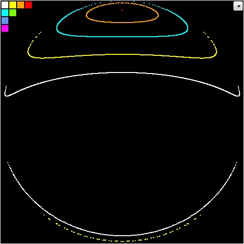
E0 = 1.0

Something very interesting is happening here! The area between inphase and antiphase motions is splitting up in many different attractors of high periodicity. The broadening of the band between two magenta attractors gets larger. Although the system still is not acting chaotic, its motions are getting more and more complex.

E0 = 1.2

Chaos has definitely entered the system. Whereas previously every motion was related to a periodic state of the system, now there is an area, visualized by the points in cyan, which has no center anymore. If the pendulum starts at some point in that area, the next point can show up anywhere in the same area. Likewise, if you start two simulations at two points in tight neighborhood, their trajectories will diverge very soon. This strong sensitivity to initial conditions is the predominant sign of (deterministic) chaos.

E0 = 1.5

As you might have expected, the region of chaotic motions gets larger and the attractors for periodic motions get smaller. Interestingly the antiphase point splits into two points.

E0 = 1.9

The large antiphase attractor completely divided into two parts and the other attractors again are getting smaller and some even disappeared.

E0 = 2.3

Now all of the attractors that showed up when the energy was raised, have disappeared and only the inphase and antiphase attractors remain.

But also a new attractor came into the system, and that's an interesting one. Remember that when the system has a total energy of 2, the lower mass is exactly on top of the upper mass (but then has no velocity anymore, because otherwise the total energy would be greater than 2). And since now the total energy is 2.3, there is enough energy for the lower mass to pass this upper position. So there is a new kind of motion which hasn't been there before: rotation.

And indeed, if you start a simulation at the center of the new attractor (in magenta), the lower mass will exactly finish a rotation cycle, when the upper mass has finished an oscillation.

E0 = 2.9

The new rotation attractor is gone again and the also the inphase and antiphase areas are getting less attractive. Chaos rules the world and the remaining attractors show up as tiny islands in a ocean of disorder.

E0 = 3.0

The antiphase periodic motion has been swallowed up by the ocean and only the inphase attractor fights with a brave heart against the surging billows of chaos.

E0 = 4.0

This is again an interesting situation. E0 = 4 means, that the upper mass is able to reach the point above the pivot, but without any velocity. So it's just before the upper pendulum can also start to rotate. Still the inphase periodic motion is stable, although its attractor gets smaller again.

You will also notice that the overall shape of the phase state distribution is changing. Whereas previously all Poincaré points have been contained in more or less a circle, now there is a tip at both ends of the x axis.

Remember that the x axis of the Poincaré diagram is showing the angle of the upper pendulum. As being said before, this angle can now reach its maximum value which is 180 degrees. The y axis is showing the angular momentum and that must be 0 if the pendulum reaches its maximum angle, otherwise the energy would be larger than 4. Although the pendulum shows the same behavior also for lower energies, the situation comes to a head at the energy of 4.

E0 = 4.5

Now that the upper pendulum is also able to perform rotations, chaos is the sole ruler of the world. Even our brave inphase oscillation, that has accompanied us from the beginning, eventually sank beneath the waves. There is no stable periodic motion anymore.

Note that on the far ends of the x axis, where the angle Θ1 is 180 degrees, now there is enough energy for an angular momentum L1. That's why there are points at both positive and negative y at these maximum x values.

E0 = 5.0

Land in sight! A new attractor rises from the sea! But in fact it is not new but showed up once at the energy of 2.3: it's the one where the lower pendulum completes a rotation, when the upper one completes an oscillation. It's quite astonishing that this very motion now shows up again.

E0 = 8.0

The green attractor gets more influence and a tiny new attractor appears in white. Remember that the maximum potential energy of our pendulum is 6. This energy is required to move both masses above the pivot. Now that the total energy is larger than 6, the pendulum can reach this position and still has enough energy to move on. And exactly this happens at the new attractor. Both pendulums are rotating with the same frequency but in different directions. This motion looks great in the 2D and 3D views and it's really surprising that it is stable!

E0 = 9.7

More rotation attractors appear. This time also in the former inphase region. If you start a simulation at the upper white attractor, you will see both pendulums rotating in the same direction.

You should definitely try out the lower red and yellow attractors! The pendulums are rotating in different directions, and whereas for the white attractor the frequencies are the same, their ratio is now 1:2 (red) and 2:3 (yellow). The resulting motions look really great!

E0 = 13

Chaos gets pushed back and more attractors appear. The blue one belongs to an antiphase rotation with a frequency ratio of 1:3. In the inphase region the white attractor shows an interesting figure. While the upper part belongs to the strictly stretched rotation, another periodic motion splits off with the lower pendulum oscillating around the stretched position.

E0 = 20

The region of chaos is getting smaller again and although no new attractors appear, their influence gets larger.

E0 = 60

Some attractors have disappeared and quasiperiodic rotations are gaining the upper hand. Chaos is definitely on the retreat. Check out the upper attractors in red!

E0 = 200

Chaos completely disappeared from the lower antiphase region which is now governed by quasiperiodic motions. Only a small chaotic band remains in the inphase region.

E0 = 4000

At this very high energy chaos is gone! All attractors besides the one for the stretched rotation are getting smaller.

E0 = 64000

Now that the total energy is again 16 times larger than before, more or less a single periodic motion remains (the dominant white attractor). The red and green attractors have a very small area of influence and they will disappear when the energy gets even larger.

Summary

The motions of a planar double pendulum can be divided into three categories, which are characterized by the total energy of the system:

1. When the energy is too small for rotations, the phase space is dominated by quasiperiodic oscillations with two strictly periodic states: inphase and antiphase oscillation.
2. If then the energy gets larger, but still is not large enough for both pendulums to easily rotate, first new periodic motions appear which turn into chaos soon. The system is highly sensitive to initial conditions.
3. Once the energy is larger than the maximum potential energy, periodic rotations appear. Chaos steps back and in the end a single periodic rotation remains. All other states are quasiperiodic.

The Code

Let me give you some details about the code for this rather simple WPF application from bottom to top. This section just covers the main classes and I hope that the helper classes speak for themselves.

Class PendulumData

This is the mathematical ground of the code. The class holds the four initial state parameters of the double pendulum and calculates the progress in time by a certain kind of numerical integration, the last point approximation (LPA). The LPA is easier to use than the Runge Kutta technique and is acceptable for our system as far as errors are concerned.

The state parameters are q1, q2, w1 and w2 , where q stands for angle and w (that is omega) for angular velocity. To initialize the data model using these parameters, just call Init(double q01, double q02, double w01, double w02). This method will calculate the corresponding angular momentums l1 and l2 and the total energy e0.

Besides the above Init() method, which let's you choose the physical state of the pendulum in a completely free way, there is another one, which is used when the pendulum should start with the Poincaré condition. The signature of this method is Init(double e00, double q01, double l01), so it gets the total energy plus the angle and angular momentum of the first mass. Since the Poincaré condition means that q2 = 0 and w2 > 0, the method can now calculate l2 by solving a quadratic equation, which then leads to w1 and w2.

The pendulum's movement is calculated by method Move(int numSteps). The numSteps parameter allows a calling method to check for conditions when the simulation should be terminated without slowing down the performance too much. Its value is just used in a for loop which repeats the actual calculation by the given number.

This actual calculation is the last point approximation and works like this:

1. The four state parameters q1, q2, w1 and w2 lead to angular accelerations a1 and a2 for the two masses (by means of the Lagrangian mechanics)
2. Each angular acceleration leads to a change of the corresponding angular velocity. If we choose a small enough time interval dT, we can do the linear approximation w1 += a1 * dT (and the same for w2)
3. Now the angular velocity leads to a new angle itself, which we can also calculate with q1 += w1 * dT (and again for q2)
4. With these new state parameters we can go back to the first step and calculate new accelerations

The time interval dT is crucial for the validity of the above linear approximations. If we choose it to large, the system will not behave 'natural' and the results will be incorrect. Choosing it very small will reduce the errors but slow down the performance of our simulation. So there needs to be some check which tells us, if the simulation is still valid after a certain amount time.

It turns out that the total energy allows us to do this test. As being said, the total energy of our system is constant, so if we calculate that energy from time to time, we can compare it with the initial energy, and if the difference is small enough (let's say < 0.1%), we can assume that the simulation is OK. And this is done at the end of the Move() method. The difference is stored as percentage value in the variable dE.

The time interval is recalculated each time the energy is set in one of the Init() methods. Higher energies need a smaller dT to come to the same relative error. It is chosen in a way that dT is 1e-6 if the energy is 1.

Before calculating new state parameters, the Move() method also checks, if the pendulum is in the Poincaré condition. This cannot be done by testing q2 against 0 directly, because the stepwise integration will not lead to this value exactly. But if we store the value of q2 in a variable q2old before doing the integration, we can identify the Poincaré condition (q2 = 0 and w2 > 0) by this expression: (q2old < 0 && q2 >= 0 && q2 <= Math.PI / 2). If the expression is true, two things happen:

1. A linear interpolation is made to calculate the state of the system when q2 exactly was 0. This state is stored as a new PoincarePoint in a list.
2. An event is raised, which tells an observer, that a new point is added to the list (NewPoincarePoint).

Class Simulator

This class has PendulumData instance and methods to start and stop the simulation, which is performed in its own thread using a BackgroundWorker. This ensures that the UI is responsive while doing the time consuming simulation.

The simulation itself is done in an endless loop of the Worker_DoWork() method. Inside of this loop the pendulum is moved a thousand times before a check is made if the loop should be terminated. A counter is used to show the calculation speed in the UI later.

If the Poincaré condition is detected inside of the Move() method, the event handler Data_NewPoincarePoint() is called. This handler just calls the ReportProgress() method of the background worker, which in turn calls the handler Worker_ProgressChanged(). This last method is executed in the UI thread, whereas the ones before are executed in the background thread. So we can modify the UI elements in this method.

Since the Simulator class does not know about UI elements, it also just raises an event, which will be handled in the UI. The name of this event is the same as the one in the PendulumData class: NewPoincarePoint.

Class PendulumModel2D

This UI element shows a 2D model of the pendulum and lets you modify the initial parameters of a simulation. It's just a WPF Canvas with some lines, curves and circles which are positioned and rendered on the basis of a PendulumData instance in the Update() method. This data model is not an instance on its own, but just a reference to the instance inside of the Simulator class.

It should be noted that this UI element does not modify the data model, but just reads the values of Q1, Q2, W1, W2, A1 and A2 to show positions, velocities and accelerations of the pendulum bobs.

There is also a method called NewPoincarePoint(), which changes the color of the lower mass to red for 120 ms. This is called when the Poincaré condition is true during a simulation.

Class PendulumModel3D

There are many ways to construct a double pendulum in the real-world, and one of them could look like this funny one. I did not give it a real try, but I guess it would work.

The 3D model is created with the WFTools3D library, which you can find here on codeproject and on github.

This UI element also has a reference to the data model of the simulator class, and it just reads Q1 and Q2 to show the current state of the pendulum in the Update() method.

Note that the 3D view is interactive. You can move the camera to any position and even fly through the scene with keyboard and mouse commands that you'll find in the previously mentioned articles.

Class PoincareMap

The map is implemented as a WPF Border which has an Image as child element. The Source of this image is set to an instance of the WriteableBitmap class.

Adding points to the bitmap is done with the great extensions library WriteableBitmapEx, which you can find here and on github.

Just like the 2D and 3D pendulum models, the map reads the data of the current simulation from a reference to the data model of the simulator. To add more simulations to the map, method CloneData() is used. This method copies the current data model and adds the copy to an internal list, which is rendered (together with the current data model) in the Redraw() method.

The zooming functionality is implemented by a PixelMapper class, which holds a stack of linear transformations to map data values to screen coordinates.

Class MainView

This WPF UserControl puts it all together! It has a simulator and all the view models, controls and event handlers to control the simulation. This makes it easy to add the whole functionality into your own application.

Class MainWindow

This WPF Window just embeds a MainView and takes care for the positioning of the application window. I hate applications which do not remember their last position!

Points Of Improvement

If you want to study the long term behavior of the double pendulum on your own, you will need to permanently store the simulation data. The code presented here is a subset of the code that I used to create the Poincaré diagrams shown above. It takes days and weeks for a single computer to create these maps, so you want to be sure that the work is not lost, when the next power failure puts your machine to death.

You can speed up things by using additional threads to calculate more than one simulation at a time. Modern computers have 4, 8 or even 16 CPUs, which are sleeping most of the time! When I started this project 20 years ago(!) that situation was different, and there was only one CPU per machine and multithreading was hardly known (at least to me :-). Fortunately I was working at a software company and so I was able to do something I call multimachining. When our daily work was done, I started the simulation on every computer I could lay my hands on. Same for the weekends!

It is also interesting to add more views to the data, e.g. a 3D view which shows the phase space trajectory in a subset of the 4D space. The next picture shows the path of a rather complex periodic motion in the (Q2, L2, L1) space. The white curve represents the path and the other two are projections onto the coordinate planes:

You can also add a third dimension to the Poincaré map. Remember that this diagram is showing L1 versus Q1 and that L2 can be calculated from the total energy. As a result the 3D Poincaré points are located on a so called energy shell, which is visualized here:

The End

I hope you enjoyed reading this rather long article as well as I did enjoy writing the code for this simple but remarkable dynamic system. If you are interested in the simulation data that I have gathered so far, just drop a note and we will find a way to transfer the 65 MB.

Happy coding!

History

5-May-2016: Initial upload