
Fundamentals of Image Processing - behind the scenes
4.97/5 (273 votes)
The article presents idea and implementation of fundamental algorithms in image processing.
Introduction
Image processing algorithms have became very popular in the last 20 years, which is mainly due to the fast extension of digital photography techniques. Nowadays, digital cameras are so common that we even do not notice them in our daily life. We are all recorded in the subway, airports, highways - image processing algorithms analyze our faces, check our behavior, detect our plates and notice that we left our luggage.
Moreover, most of us were using image processing algorithms in software like Photoshop or GIMP. To receive interesting artistic effects.
But, however advanced these algorithms would be, they still rely on fundamentals. In this article we are going to present the basic image processing algorithms that will help to understand what does our graphics editor software calculates behind the scenes.
From basics to infinity
First Lady of the Internet
Before we begin our journey through image processing methods, we should know a brief story of certain model and her photo.

For those involved in image processing, this photo is well known. The image above shows Swedish model Lenna Soderberg (nee Sjööblom). It was originally printed as Playboy centerfold in November 1972.
The photo was firstly used in 1973 by accident and since that time it has became the most important photo in image processing and compression researches.
Image representation in digital world
A world that we observe everyday is continous. That is the way, how our eyes perceive images. To capture the analog image on a digital media, it needs to be sampled and quantized - in a one word, it needs to be digitalized.
Sampling
As a result of sampling continous 2D signal (image) we receive discreet 2D signal with defined number of rows and columns. The point (element) at the intersection of given row and column is named pixel. Sampling original image is a lossy operation - the quality of sampled image depends on the assumed level of sampling.


Fig. Results of using different levels of sampling.
Quantization
Quantization is the operations that answeres us what is the value of each pixel in our dicreet image. Typical levels of quantizations are 2, 64, 256, 1024, 4096, 16384. For example if we use 1024 levels of quantizations that means that the value of each pixel is a natural number in range 0 to 1024.


Fig. Results of using different quantization levels.
Color
The last information that we need to add to our digital image is a color of each pixel. The most popular color model is a cubic RGB model. Red, green and blue are the colors from which we can create any other. In RGB model each image pixel is described by three values - saturation of each color.

Another common color model is HSV. HSV model describes color using three components: hue, saturation and value. The model can be considered as a cone, which is based on color palette.

In printing process the most popular color model is CMYK, which stands for the names of the four primary colors: cyan, magenta, yellow and key (black). In printing process each of color element is joined to give a final color.

Histogram
Image histogram is a statistical information of times that each color or brightness level occurs in image. Histogram tells us a lot about the image - not only about its brightness and contrast. Using histogram we can deduce if the image details have been correctly captured and stored.
When analyzing color image we receive histograms for each color (RGB). Single histogram can be generated for greyscale image.


Fig. Histograms of color and greyscale images
Image representation in frequency domain - image spectrum
Discrete Fourier Transform
Image should be treated as any other signal that is transfering information in discrete spatial domain. Due to this we can transform it to a frequency domain.
Discrete forward and inverse Fourier Transform (forward DFT, inverse DFT) are described with formulas:
From above we can notice that F(0,0) refers to static component. Futher from this point, higher frequencies are represented. We need to remember that each complex value may be presented as magnitude and phase:
Although the information are carried only by the magnitude, we still need to remember about phase component to be able to calculate inverse transform. To present magnitude as a bitmap we also need to normalize its values. Usually we normalize with a logarithmic scale:


Fig. Magnitude of image DFT.
It is customary to assume that the static component is shown in the middle of the image. Therefore, we need to perform spectrum shift:
Instead of making shift operations may be performed on the original. Note that:

Fig. Magnitude of image SDFT. We can see that magnituded reaches non-zero values through all frequency range, however static component is dominating. We can also notice, that three directions (vertical, horizontal and sloping in 45º) are dominating in image.
A. 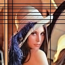

B. 

C. 

D. 

Fig. How a change in the image affects its spectrum. A. Adding additional horizontal and vertical lines enhanced these directions in spectrum. B. Adding low-level noise resulted in suppression of the main directions of the visible spectrum. C. Adding high-level noise caused bluring magnitude values on all frequencies. D. Rotating image resulted in rotating main directions in spectrum.
Basic image convertion
Color model change
Formulas given below show the idea of convertion between three most common models of colors.
RGB to HSV
Auxiliary variables:
Final calculation:
HSV to RGB
Auxiliary variables:
Final calculation:
1. If IH(x,y) is between 0º and 60º
2. If IH(x,y) is between 60º and 120º
3. If IH(x,y) is between 120º and 180º
4. If IH(x,y) is between 180º and 240º
5. If IH(x,y) is between 240º and 300º
6. If IH(x,y) is between 300º and 360º
RGB to CMYK
RGB color elements normalization:
The calculation of the individual CMYK components:


Fig. Cyan, Magenta, Yellow and Key layers
CMYK to RGB
The calculation of the individual RGB components:
Color image to greyscale
There are few algorithms that creats greyscale image from color one. The difference between them are the methods of converting three color components in to one - brightness.
Average method
The final product is average of each color comonent.
Lightness method
The final product is average of maximum and minimum of color components.
Luminance method
The most popular method which is designed to match our brightness perception. This method is using weighted combination of color components.


Fig. Result of greyscaling operations (from left: average, lightness, luminance)

Fig. The difference between greyscaling operations.
Greyscale image to black and white
Converting greyscale image to black and white is nothing else than verifing if each pixel brightness value is below or above assumed threshold T.


Fig. Converted images using different thresholds (from left: 100, 128, 156)
Negative
In calculating negative image we calculate complement of each pixel. This is a reversible operation, i.e. as a result of double use this function, we will receive original.
For color images, each color element should be calculated using formula above.


Fig. Image positive and negative
Inverse
Calculating inverted image comes to calculating new value of each pixel which it is located symmetrically with respect to conversion point.


Fig. Inverted greyscale image (conversion point 128)


Fig. Inverted black and white image (conversion point 128)
Addition
Two images addition is as simple as two numbers addition:
Due to available brightness values additional condition needs to be check:

Fig. Image A

Fig. Image B
Fig. A + B
Subtraction
When subtracting two images we need to mind which image is minuend and which is subtrahend:
The same as in images addition available brightness values condition needs to check:

Fig. Image A

Fig. Image B

Fig. B - A
Horizontal and vertical flip
These operations creates image mirror reflection:
Horizontal
where W is image width.


Fig. Horizontal flip
Vertical
where H is image heigth.

Fig. Vertical flip
Contrast stretching
Contrast stretching is one of the histogram-based operations. We use it to brighten orginal imag if its histogram is mostly located on the left side. The idea is to stretch (increase) cantrast over the whole available range.
The operation is described by formula:
where IMIN and IMAX are minimum and maximum brightness values in image, MIN and MAX are minimum and maximum available values in output histogram.


Fig. Orginal image


Fig. Contrast stretched (Min = 0, Max = 255)


Fig. Contrast stretched (Min = 50, Max = 255)
Histogram shifting
Histogram shifting operations are used for brightening or dimming. It is noting more but only adding offset value to each pixel:


Fig. Original image


Fig. Histogram-shifted image (offset = 75)
Histogram equalization
Histogram equalization method is used in case of low contrast images. The idea is to spread image histogram to enhance contrast and highlight the difference between the image subject and the background.
Operation is described with formula:
where H is available levels of brightness (mostly it is 256), and pi is the probability of occurrence of pixel with specific brihtness:
where hist(i) donotes the number of pixels with i-level of brightness (i element of histogram vector) and N denotes total number of pixels in image.
This operation is very often used in projectors as a method of improving diplayed image.


Fig. Original image


Fig. Histogram equalized image
Logaritmic scaling
Logaritmic scaling operation normalize pixel values by replacing with its logarithm. As a result lower values are enhanced and whole histogram streched.
Usually we use 10 base or natural logarithm. The operation is described with formula:


Fig. Original image


Fig. Logaritmic scaled image
Workspace change
Workspace change operations (sometimes named as canvas change) consist of changing (reduce or expand) image size without changing original image pixels' values.
First thing we need to define is range of interest anchor position. In the image croping operation anchor position defines position of new crop, in the image complement operation anchor position defines original image position in new size.

Fig. Anchor positions
Crop
In image crop oparation start point (x1; y1) of new range of interest needs to be calculated depending on assumed anchor position.
Denote by W and H original image dimensions (width and height) and by w and h cropped image dimensions. Then:
Middle
West
East
North
South
North - West
North - East
South - West
South - East
Finally, for each pixel of new image we take corresponding pixel of original image:

Fig. Original image (225 x 225 px)


Fig. Cropped images 50 x 50 px (from left anchor positions: west, middle, north, north-west, north-east, south, south-west, south-east, east)
Complement
In image complement oparation start (x1; y1) and end (x2; y2) points of new range of interest need to be calculated depending on assumed anchor position.
Denote by W and H complemented image dimensions (width and height) and by w and h original image dimensions. Then:
Middle
West
East
North
South
North - West
North - East
South - West
South - East
Finally


Fig. Original image (125 x 125 px) and complemented image (150 x 150 px) with center anchor position.
Resampling
Resampling operations consist of changing the number of pixels in the processed image to resize it, change proportions or rotate.
Resize
In resize issue we want to change image width and height, with or without saving it's proportions. Lets denote original image width and height as W, H and desirable width and height as WO and HO.
So the transformation ratios are:
Nearest neighbour
This is the simplest method to resize image.
For each pixel we need to calculate its equivalent in the original image:


Fig. Image resize using nearest neighbour method (from left original 128x128, resized 256x256 and 50x50)
Bilinear interpolation
The disadvantage of nearest neighbour method is leaving jagged edges in the picture. This problem is devoid of method that involves the interpolation of the surrounding pixels.
For each pixel we need to calculate the center of range of interest in the original image:


Fig. Image resize using bilinear interpolation method (from left original 128x128, resized 256x256 and 50x50)

Fig. Comparison of both methods
Rotation
To rotate image we need to select the center of rotation (xc, yc) - the point relative to which we will transform image. This will usually be the center of the original image, but presented transformations assume any point selection.
The Pixel (x, y) of an output image is the pixel (xA, yA) of the original image, calculated with the following equation:


Fig. Image rotation (from left 30º, 45º, 60º), image center is a center of rotation.

Fig. Image rotation 30º, center of rotation in point x=25, y=25
Linear filtration
Linear filtration is nothing but a frequency filtering, whereby certain frequencies are left unchanged, and the other are suppressed. The operation of filtration can be performed both in the frequency as well as in spatial domain.
While in terms of computational complexity, performing the filtering in the spatial domain is much easier (no need to calculate a forward and inverse Fourier transform), it must be remembered that frequency filters are described in the frequency domain and is not always an easy way to find a kernel such a filter in the spatial domain.
Convolution in spatial domain
In spatial domain frequency filters are represented by real values matrices. To receive output image we need to calculate two-dimensional convolution of original image with filter mask.
3x3 dimension filter can be presented as a matrix:
where the center element x5 corresponds to position of output pixel calculation. The filter mask 'travels' through all rows and columns of original image with operation:
For color images we need to perform the above operation for each layer.
Lowpass filters
Low pass filters (sometimes named as average filters) suppress the higher frequencies and leaves lower ones. It is built by combining two one-dimensional filters.


Fig. 1D and 2D low pass filters. Blue color indicates pass bandwidth.
In fact, low pass filtering is calculating average value of each output filter. Unwanted effect is image bluring. Examples of low pass filters masks are:


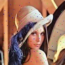


Fig. Low pass filtartion (from left; original, LPF1, LPF2, LPF3, LPF4)
Highpass filters
High pass filters (sometimes named as sharpen filters) suppress the lower frequencies and leaves higher ones. It is built by combining two one-dimensional filters.


Fig. 1D and 2D high pass filters. Blue color indicates pass bandwidth.
The purpose of these filters is sharper edges and small details (high-frequency counterparts in the spatial domain). In addition to the desired effect, high pass filter is also strengthened noise. Examples of high pass filters masks are:


Fig. Hihg pass filtration (from left: original, HPF1, HPF2, HPF3, HPF4)
Gaussian filter
Similarly to the low pass, Gaussian filter smoothes image removing noise, small details and blurs edges. The difference is in filter mask kernel, which in the case of this filter takes the form of a two-dimensional plot of gaussian function.

Fig. 2D Gaussian function.


Fig. Gaussian filter 9from left: original, GF1, GF2, GF3)
Non-linear filtration
Non-linear filters are different class of filtration. In contrast to the linear filters we can not use convolution to calculate the output image (and thus we can not process images in the frequency domain). Due to this non-linear filtration algorithms are slower then linear ones. However, the use of non-linear filters leads to good results in the initial image processing.
Median filter
Median filters are the most popular non-linear filters. In this operation to calculate new value of each pixel we take the median value of pixels in nearest neighborhood. The range of nearest neighborhood is defined by filter mask size. Using larger sizes of the mask causes larger bluring of the output image.
The next steps of median filtering with 3x3 mask are:
1. Get nearest neighborhood pixels values:
2. Order these values from minimum to maximum:
3. Calculate value of new pixels as median of the list above, which is s5 element:


Fig. Median filtration of color image (from left: original image, mask 3x3, mask 5x5)
Median filtering is used for impulse (salt & pepper) noise cancellation. Unlike lowpass filter, median is less damaging in smoothing step changes of brightness values.


Fig. Impulse noise cancellation using 3x3 median filter
Signal-dependent rank ordered mean filter (SD ROM)
The disadvantage of median filter is changing value of the pixel even if it is not corrupted. In result our image gets blurred without attention to if it was noisy or not. The idea of SD ROM filter is to check wheater the pixel is corrupted an calculates its new value only in that case.
The next steps of SD ROM filtering with 3x3 mask are:
1. Get nearest neighborhood pixels values:
2. Order these values from minimum to maximum:
3. Calculate ordered mean value:
4. Calculate ordered subtraction vector:
where for declared mask dimension 3 x 3, i = 1, 2, 3, 4.
5. For each element in ROD vector check the condition:
where
and T is a vector of given thresholds, where
If any of conditions from point 5 is true we can suppose that pixel (x, y) is corrupted and we change its value to ROM(x,y). Otherwise we leave its value as in original image.
For general case of N x N mask our
1A. Nearest neighborhood pixels values matrix would be N x N
2A. R vector would have N2 - 1 elements
3A. Ordered mean value calculation would be:
4A. Ordered subtraction vector calculation would be:
where i = 1, 2, 3, 4, ..., (N^2 - 1) / 2.
5A. We need to declare N2 - 1 elements of thresholds vector


Fig. SD ROM filtration of color image (from left: original image, mask 3x3, mask 5x5)


Fig. Impulse noise cancellation using 3x3 SD ROM filter
Fig. Comparison of using median and SD ROM filters in noise cancellation.
Kuwahara filter
Kuwahara filter is another example of smoothing operator that is not bluring image edges (unlike median filter) but in contrast to SD ROM filter, it changes value of each calculated pixel.
To calculate value of pixel p(x,y) our range of interest is nearest neighborhood with dimension (2N-1) x (2N-1) where N denotes size of Kuwahara filter. For N = 3 we receive range of interest:
In nest step we divide mask above to four smaller, each in dimension N x N:
For each mask we calculate mean value and variance:
New value of p(x,y) is a mean value of the mask with lowest variance.


Fig. Impulse noise cancellation using size 3 Kuwahara filter
Morphology filtration
Morphology filtration should be treated as a completely separate area for image processing. It is mainly used for pre-processingto prepare the image for further operations. Typically morphology methods are used in the processing of binary images, but can also be successfully used in greyscale image processing.
However, processing of color images using morphological filters is not so easy task, due to the strong correlation between individual color components of a pixel - filtration of each color layer and further connecting does not give us a rewarding result.
This article will focus on the most common use of morphological operations for the processing of binary images
Erosion
The purpose of this filter is the depletion of the compact object in the image to eliminate unwanted connections with neighboring objects or unwanted jagged edges of the object.
In this operation to calculate new value of each pixel we take the minimum value of pixels in nearest neighborhood. The range of nearest neighborhood is defined by filter mask size.
The next steps of erosion filtering with 3x3 mask are:
1. Get nearest neighborhood pixels values:
2. Calculate value of new pixels as a minimum value of matrix above.


Fig. Image erosion (from left: original image, erosion with mask 3x3, erosion with mask 5x5).
Dilatation
The purpose of this filter is bold object surface to eliminate pits.
In this operation to calculate new value of each pixel we take the maximum value of pixels in nearest neighborhood. The range of nearest neighborhood is defined by filter mask size.
The next steps of erosion filtering with 3x3 mask are:
1. Get nearest neighborhood pixels values:
2. Calculate value of new pixels as a maximum value of matrix above.


Fig. Image dilatation (from left: original image, dilatation with mask 3x3, dilatation with mask 5x5).
Opening
As it can be seen at the figure showing effects of erosion filtration, using appropriate mask dimension resulted separation of four objects. However, the unwanted effect is reducing the area of each.
To avoid such situations, often instead of using erosion filtration, we use opening operation, which is dilatation of the image filtered with erosion mask.


Fig. Image opening (both erosion and dilatation with mask 5x5)
Closing
The opposite effect, to that observed in erosion, can be seen in the result do image dilatation. Pits were lost, but the object filed has been enlarged.
To avoid such situations we can use closing operation, which is erosion of the image filtered with dilatation mask.


Fig. Image closing (both dilatation and erosion with mask 5x5)
Skeletonization
The most common definition, or rather purpose, of the skeletonization is to extract a region-based shape feature representing the general form of an image object. As a result we receive the medial axis of the given object.
The object's skeleton is not unambigous - two different shapes can have the same skeleton.

Fig. Binary images and its' skeletons
The skeletonization algorithm can be separeted into three steps:
Step 1. Image prepartion
If we assume binary image with pixel values of 0 (black) and 1 (white), this step can be omitted. Otherwise, all it needs to be done in this step is to normalize pixels' values to receive zeros and ones.
Step 2. Calculate recursively medial axis direction
To calculate next values we follow formula below:
Calculation should be repeated until no more changes in table can be observed.
Step 3. Skeleton lines isolation
The skeleton lines can be calculated with formula:
Edge detecting filtration
Typical case in image processing is edge detecting - very often used in medical image processing. Edge detecting in spatial domain can be divided into operations using directional or non-directional filters.
Directional filtering necessitates double of the mahematical operations and futher combining the results. This is not required in the case of non-directional filters.
Edge detecting filtration can be also called as derivative filtration or gradient filtration, because it is based on determining the derivative of original image. Usually, the occurrence of the edge is a sudden change in the brightness level of pixels, which strongly reflects on the values of the first (or next) derivatives.
Sobel filter
Sobel filter, or Sobel operator, is an example of diractional filter.
It detects horizontal edges with mask:
and vertical with:
At the end we combine results
which can be approximated with


Fig. Edge detecting on color image using Sobel filter
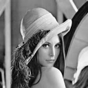

Fig. Edge detecting on greyscaled image using Sobel filter


Fig. Edge detecing on unnatural black and white image using Sobel filter
Prewiit filter
Prewitt filter, or Prewitt operator, is an example of diractional filter.
Horizontal mask:
Vertical mask:


Fig. Edge detecting on color image using Prewitt filter


Fig. Edge detecting on greyscaled image using Prewitt filter


Fig. Edge detecing on unnatural black and white image using Prewitt filter
Laplace filter
Filtration using Laplace masks is calculating second derivative. These are examples of non-directional filters. Examples of Laplace masks are shown below:


Fig. Edge detecting on color image using Laplace filter


Fig. Edge detecting on greyscaled image using Laplace filter


Fig. Edge detecing on unnatural black and white image using Laplace filter
Art filtration and processing
Color filtration
It is a very simple algoritm, which can replace the use of physical filters applied to the camera lens.
Natural light (consisting of different wavelengths corresponding to different colors) passing through a color filter is losing (suppress) selected wavelengths. As a result only selected colors (wavelenghts) are reaching image sensor.
For example, when using magenta filter, magenta color is build from red and blue, only red and blue components will pass - the green will be stoped.


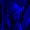


Fig. Color filtration (filters color from top left: cyan, magenta, yellow, cyan-magenta, magenta-yellow, yellow-cyan)
Gamma correction
Gamma correction is used to reduce or increase contrast.
For greyscale images it is given with formula:
where INOR denotes normalized image value to range 0 - 1.
For color images, the operation above should be repeated for each color component.


Fig. Gamma correction (from left: 0.25, 0.5, 0.75, 1.5, 2)
Sepia
Sepia toning is one of the techniques used in traditional photographic processing. This technique was used in order to increase the lifetime of photographic printing. As a result, image took on a brown color.
To get the same effect with a digital image proccessing perform two operations: firstly we convert color image to greyscale, then we change RGB values of each pixels using formula below:


Fig. Image in sepia with different levels (from left: 10, 20, 30, 40, 80)
Color accent
This artistic technique is based on accenting (leaving) only selected colors on the image, whereas all others are converted to greyscale.
To perform this we will use HSV color model instead of the RGB model. It is much easier because in HSV model we can focus only on one color parameter - hue. Of course, the hue value can vary, that is why we should assume a range of acceptable changes.
Lets denote values h, which is hue of the color we want to accent, and r, which is acceptable range. We can calculate values:
These values can be in the relationship:
1.
In this case we leave pixel value if additionally:
2.
In this case we leave pixel value if additionally:


Fig. Color accent examples
Layers
Layering is a very common operation in image processing. As a result we receive image which is combination of two inputs (background and layer).
To calculate output pixel we use technique named alpha blending, given with the formulas below:
Finally we calculate new alpha factor for (x, y) pixel:


Fig. Adding layers examples
Tilt shift
Tilt shift technique is known from traditional photography, where by using special objectives with possibility to shift optical axis we change image perspective. At the end we receive image with elements on it that seems to be a model.
In digital image processing we can obtain the same result without without the need for specialized photographic equipment.
The tilt shifted image is divided into three parts: two of them are blurred, middle one stays sharp as in an original image. The ratios can vary and in our example we will use technique half-of-half, where top blurred part is half of an original image and bottom blurred part is half of the left half.

Fig. Tilt shift image structure
To blur image we will use one-dimensional gaussian filter. Bluring can be made either in horizontal or vertical directions. Gaussian function is denote below:
where:
L - is defined function value for blurring in close proximity to sharp part (ex. in range 0.05 - 0.15)
S - is defined function value for blurring in far proximity to sharp part (ex. in range 5 - 7)
n - is distance between calculating pixel and sharp part
N0.5 - is height of larger blurred field (in vertical blurring)
For each pixel that should be blurred we perform calculation (vertical bluring):
To make the formula above be countable we need to considered as negligible low values of gaussian filter (ex. values below 0.005).


Fig. Tilt shift effect.
Image blurring
Image blurring opertion is quite similar to tilt shift filtration. We can use the same gaussian function as blur operator. The difference is in output image structure, where we define the center of sharp ring and its radius. All pixels outside of this ring should be blurred.

Fig. Blurred image structure
The distance between specific pixel and the center of ring is calculated from formula below:
If r > R we use gaussian filter.

Fig. Blurred image (center in point 250x180, radius 80)
Blurred background
Interesting effect we can receive when placing image (rotated or not) on background created from the same image but blurred. Following operations are:
1. Blur image using Gaussian filter (this step can be repeated even two or three times) - this blurred image is going to be our background
2. Complement image (original one) with white frame
3. Complement result from 2 with transparent background (to get rid of "dog-ears")
4. Rotate result from 3 (if we don't want to rotate foreground we can miss step 3 and 4)
5. Add foregroung image as a layer to background.


Fig. Blurred background effect
Polaroid frame effect
Polaroid frame effect is similar to blurred background composition. We can receive it by omitting backgound creation and enlarging bottom frame width.
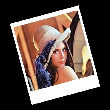
Fig. Polaroid frame effect
Pen sketch
Pen sketch effect can be received by combining two operations: edge detecting and black and white with inversion over defined intensity.
We can also use SD-ROM algorithm to dispose of smaller artifacts without bluring edges.


Fig. Pen sketch effect (Laplace edge detecting, black and white with inversion over 80, SD-ROM)
Charcoal sketch
Charcoal effect can be received in similar way to pen sketch. Addtionally we can start and finish with smoothing image (median or gaussian filter). Instead of black and white method we can use image inverse operator.


Fig. Charcoal effect (Sobel edge detecting, inverse with value 80, median smoothing with size of 5)
Oil paint
To receive oil paint effect we need to reduce available levels of pixel intensity. Normally, each pixel is descibed by 256 levels of intensity - for oil paint filtering we will reduce them more then 10 times.
To categorise pixel we need to consider intensities of its nearest neighbourhood in defined radius (size of oil paint filter) r. Also, lets denote L as defined levels of available intensities.
Lets denote vectors of intesity levels occurance: I - histogram of categorised intesities, R, G, B - red, green and blue colors values at categorised intensity.
For each pixel in defined by r neighbourhood we calculate categorised intensity:
and increment vectors:
Afterwards we designate maximum value of histogram I and index of its maximum value k.
Finally, we calculate new red, green and blue values as:


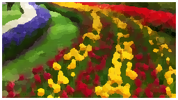
Fig. Oil paint effect (filter with radius of 7, 15 levels of color intensity)
Cartoon effect
If we additionally combine result of oil paint filtration with inverted edge detecting filtration we can receive equally interesting effect - image looking like a comic book drawing.


Fig. Cartoon efect (oil paint filter with radius of 7, 10 levels of color intensity, inverse threshold 40, Sobel operator)
Using the code
All image processing algorithms presented in this article are implemented in attached source code. To start working with FIP library simply declrae its namespace:
using FIP;
Create new object:
FIP.FIP fip = new FIP.FIP(); // many "fip's" in one line...
and start your journey in digital image processing...
Library methods calling
Histogram
To receive table with histograms:
Bitmap img = new Bitmap("781213/lena.jpg");

int[] greyscaleHistogram = fip.Histogram(img); // Greyscale histogram
int[,] rgbHistogram = fip.RGBHistogram(img); // RGB histogram
Discrete Fourier Transform
Forward Fourier Transforms:
Bitmap img = new Bitmap("781213/lena.jpg");

Complex[,] spectrum = fip.DFT(img); // Basic forward Fourier Transform

Complex[,] spectrumShifted = fip.SDFT(img); // Forward Fourier Transform with shift operation
Get Magnitude and phase:
Double[,] magnitude = fip.Magnitude(spectrum);

Double[,] phase = fip.Phase(spectrum);
Inverse Fourier Transform:
Bitmap inv = fip.iDFT(spectrum); // To Bitmap

Double[,] invTab = fip.iDFT2(spectrum); // To table
If shift operation was applied:
Bitmap inv = fip.iSDFT(spectrum); // To Bitmap

Double[,] invTab = fip.iSDFT2(spectrum); // To table
Color model transformation
Bitmap img = new Bitmap("781213/lena.jpg");

Color pixel = img.GetPixel(1, 1); // Get single pixel

Double[] hsv = fip.rgb2hsv(pixel); // Single pixel convertion from RGB to HSV
Color pixel2 = fip.hsv2rgb(hsv); // Single pixel convertion from HSV to RGB

Double[] cmyk = fip.rgb2cmyk(pixel); // Single pixel convertion from RGB to CMYK
Color pixel3 = fip.cmyk2rgb(cmyk); // Single pixel convertion from CMYK to RGB

Bitmap[] CMYKLayers = fip.CMYKLayers(img); // Get CMYK Layers form ARGB image

Bitmap[] RGBLayers = fip.RGBLayers(img); // Get RGB Layers as bitmaps
int[,,] RGBLayers2 = fip.RGBMatrix(img); // Get RGB Layers as tables

int[,] RLayer = fip.RMatrix(img); // Get red color layer
int[,] GLayer = fip.GMatrix(img); // Get green color layer
int[,] BLayer = fip.BMatrix(img); // Get blue color layer
Convert to greyscale
Bitmap img = new Bitmap("781213/lena.jpg");

Color pixel = img.GetPixel(1, 1); // Get single pixel

Color pixelGS = fip.color2greyscale(pixel); // Single pixel convertion using luminance method

Bitmap average = fip.ToGreyscaleAVG(img); // Average method of greyscaling
Bitmap lightness = fip.ToGreyscaleLightness(img); // Lightness method of greyscaling
Bitmap luminance = fip.ToGreyscale(img); // Luminance method of greyscaling
Convert to black and white
Bitmap img = new Bitmap("781213/lena.jpg");

Bitmap bw = fip.ToBlackwhite(img, 128); // Convert to black and white with threshold on 128
Bitmap bwinv = fip.ToBlackwhiteInverse(img, 80); // Convert to black and white with threshold on 80 and invert over this point
Negative
Bitmap img = new Bitmap("781213/lena.jpg");

Bitmap negative = fip.NegativeImageColor(img); // Color image negative
Bitmap negativeGS = fip.NegativeImageGS(img); // Converts to greyscale and negative transform
Inverse
Bitmap img = new Bitmap("781213/lena.jpg");

Bitmap inverse = fip.InverseImage(img, 190); // Inverse image on point 190
Image addition and subtraction
Bitmap a = new Bitmap("a.jpg");
Bitmap b = new Bitmap("b.jpg");

Bitmap c = fip.AddImages(a, b); // Add two images
Bitmap d = fip.SubtractImages(a, b); // subtract two images a - b
Horizontal and vertical flip
Bitmap img = new Bitmap("781213/lena.jpg");

Bitmap mirrorvertical = fip.FlipVertical(img);
Bitmap mirrorhorizontal = fip.FlipHorizontal(img);
Contrast stretching
Bitmap img = new Bitmap("781213/lena.jpg");

Bitmap contraststretching = fip.ContrastStretching(img); // Contrast stretching in whole range
Bitmap contraststretching2 = fip.ContrastStretching(img, 50, 255); // Contrast stretching in range 50 - 255
Histogram shifting
Bitmap img = new Bitmap("781213/lena.jpg");

Bitmap histshift = fip.HistogramShift(img, 50); // Histogram shift with threshold of 50
Histogram equalization
Bitmap img = new Bitmap("781213/lena.jpg");

Bitmap histeq = fip.HistoramEqualization(img);
Logaritmic scaling
Bitmap img = new Bitmap("781213/lena.jpg");

Bitmap logscale = fip.LogaritmicScaling(img); // Logarithmic scaling with 10-base logarithm
Crop image
Bitmap img = new Bitmap("781213/lena_cut.jpg");
Bitmap cut = fip.ImageCut(img, 50, 50, FIP.FIP.Anchor.Middle);
Complement image
Bitmap img = new Bitmap("781213/lena_complement.jpg");
Bitmap complement = fip.ImageComplement(img, 150, 150, Color.FromArgb(255, 0, 0, 0), FIP.FIP.Anchor.Middle);
Image resize
Bitmap img = new Bitmap("781213/lena.jpg");

Bitmap img2 = fip.Resize(img, 50, 50); // Image resize with nearest neighbourhood method
Bitmap img3 = fip.Resize2(img, 50, 50); // Image resize with bilinear interpolation method
Image rotation
Bitmap img = new Bitmap("781213/lena.jpg");

Bitmap rotate = fip.Rotate(img, 30); // Image rotation over 30 degrees
Linear filters examples
Lowpass filters
        /// <summary>
        /// Low pass filter
        /// </summary>
        /// <returns>Low pass filter</returns>
        public Double[,] LPF1()
        {
            return new Double[3, 3] { { 0.1111, 0.1111, 0.1111 }, { 0.1111, 0.1111, 0.1111 }, { 0.1111, 0.1111, 0.1111 }, };
        }

        /// <summary>
        /// Low pass filter
        /// </summary>
        /// <returns>Low pass filter</returns>
        public Double[,] LPF2()
        {
            return new Double[3, 3] { { 0.1, 0.1, 0.1 }, { 0.1, 0.2, 0.1 }, { 0.1, 0.1, 0.1 }, };
        }

        /// <summary>
        /// Low pass filter
        /// </summary>
        /// <returns>Low pass filter</returns>
        public Double[,] LPF3()
        {
            return new Double[3, 3] { { 0.0625, 0.125, 0.0625 }, { 0.125, 0.25, 0.125 }, { 0.0625, 0.125, 0.0625 }, };
        }

        /// <summary>
        /// Low pass filter
        /// </summary>
        /// <returns>Low pass filter</returns>
        public Double[,] LPF4()
        {
            return new Double[5, 5] {
            { 0.00366, 0.01465, 0.02564, 0.01465, 0.00366 },
            { 0.01465, 0.05861, 0.09524, 0.05861, 0.01465 },
            { 0.02564, 0.09524, 0.15018, 0.09524, 0.02564 },
            { 0.01465, 0.05861, 0.09524, 0.05861, 0.01465 },
            { 0.00366, 0.01465, 0.02564, 0.01465, 0.00366 }
            };
        }
Highpass filters
        /// <summary>
        /// High pass filter
        /// </summary>
        /// <returns>High pass filter</returns>
        public int[,] HPF1()
        {
            return new int[3, 3] { { -1, -1, -1 }, { -1, 9, -1 }, { -1, -1, -1 }, };
        }

        /// <summary>
        /// High pass filter
        /// </summary>
        /// <returns>High pass filter</returns>
        public int[,] HPF2()
        {
            return new int[3, 3] { { 0, -1, 0 }, { -1, 5, -1 }, { 0, -1, 0 }, };
        }

        /// <summary>
        /// High pass filter
        /// </summary>
        /// <returns>High pass filter</returns>
        public int[,] HPF3()
        {
            return new int[3, 3] { { 1, -2, 1 }, { -2, 5, -2 }, { 1, -2, 1 }, };
        }

        /// <summary>
        /// High pass filter
        /// </summary>
        /// <returns>High pass filter</returns>
        public int[,] HPF4()
        {
            return new int[5, 5] {
            { -1, -1, -1, -1, -1 },
            { -1, -1, -1, -1, -1 },
            { -1, -1, 25, -1, -1 },
            { -1, -1, -1, -1, -1 },
            { -1, -1, -1, -1, -1 }
            };
        }
Gaussian filters
        /// <summary>
        /// Gausian filter
        /// </summary>
        /// <returns>Gausian filter</returns>
        public Double[,] GF1()
        {
            return new Double[3, 3] { { 0.0625, 0.125, 0.0625 }, { 0.125, 0.25, 0.125 }, { 0.0625, 0.125, 0.0625 }, };
        }

        /// <summary>
        /// Gausian filter
        /// </summary>
        /// <returns>Gausian filter</returns>
        public Double[,] GF2()
        {
            return new Double[5, 5] {
            { 0.0192, 0.0192, 0.0385, 0.0192, 0.01921 },
            { 0.0192, 0.0385, 0.0769, 0.0385, 0.0192 },
            { 0.0385, 0.0769, 0.1538, 0.0769, 0.0385 },
            { 0.0192, 0.0385, 0.0769, 0.0385, 0.0192 },
            { 0.0192, 0.0192, 0.0385, 0.0192, 0.0192 }
            };
        }

        /// <summary>
        /// Gausian filter
        /// </summary>
        /// <returns>Gausian filter</returns>
        public Double[,] GF3()
        {
            return new Double[7, 7] {
            { 0.00714, 0.00714, 0.01429, 0.01429, 0.01429, 0.00714, 0.00714 },
            { 0.00714, 0.01429, 0.01429, 0.02857, 0.01429, 0.01429, 0.00714 },
            { 0.01429, 0.01429, 0.02857, 0.05714, 0.02857, 0.01429, 0.01429 },
            { 0.01429, 0.02857, 0.05714, 0.11429, 0.05714, 0.02857, 0.01429 },
            { 0.01429, 0.01429, 0.02857, 0.05714, 0.02857, 0.01429, 0.01429 },
            { 0.00714, 0.01429, 0.01429, 0.02857, 0.01429, 0.01429, 0.00714 },
            { 0.00714, 0.00714, 0.01429, 0.01429, 0.01429, 0.00714, 0.00714 }
            };
        }
Laplace filters
        /// <summary>
        /// Laplace filter
        /// </summary>
        /// <returns>Laplace filter</returns>
        public int[,] LaplaceF1()
        {
            return new int[3, 3] { { -1, -1, -1 }, { -1, 8, -1 }, { -1, -1, -1 }, };
        }

        /// <summary>
        /// Laplace filter
        /// </summary>
        /// <returns>Laplace filter</returns>
        public int[,] LaplaceF2()
        {
            return new int[3, 3] { { 0, -1, 0 }, { -1, 4, -1 }, { 0, -1, 0 }, };
        }

        /// <summary>
        /// Laplace filter
        /// </summary>
        /// <returns>Laplace filter</returns>
        public int[,] LaplaceF3()
        {
            return new int[3, 3] { { 1, -2, 1 }, { -2, 4, -2 }, { 1, -2, 1 }, };
        }

        /// <summary>
        /// Laplace filter
        /// </summary>
        /// <returns>Laplace filter</returns>
        public int[,] LaplaceF4()
        {
            return new int[5, 5] {
            { -1, -1, -1, -1, -1 },
            { -1, -1, -1, -1, -1 },
            { -1, -1, 24, -1, -1 },
            { -1, -1, -1, -1, -1 },
            { -1, -1, -1, -1, -1 }
            };
        }
Linear filtration
Bitmap img = new Bitmap("781213/lena.jpg");

Bitmap fitered = fip.ImageFilterColor(img, fip.LaplaceF1()); // Image filtration with Laplace filter no 1
Bitmap fiteredGS = fip.ImageFilterGS(img, fip.LaplaceF1()); // Image filtration (with greyscaling operation) with Laplace filter no 1
Median filter
Bitmap img = new Bitmap("781213/lena.jpg");

Bitmap median = fip.ImageMedianFilterColor(img, 5); // Median filtration with mask size 5;
Bitmap medianGS = fip.ImageMedianFilterGS(img, 5); // Median filtration with greyscaling and filter mask size 5
SD-ROM filter
Bitmap img = new Bitmap("781213/lena.jpg");

Bitmap sdrom = fip.ImageSDROMFilterColor(img); // SD ROM filtration with parameters described in article
Bitmap sdrom2 = fip.ImageSDROMFilterColor(img, 3, new int[4] { 30, 40, 50, 60 }); // SD ROM filtration with given parameters

Bitmap sdromGS = fip.ImageSDROMFilterGS(img); // SD ROM filtration with parameters described in article additionally greyscaling operation

Bitmap sdrom2GS = fip.ImageSDROMFilterGS(img, 3, new int[4] { 30, 40, 50, 60 }); // SD ROM filtration with given parameters additionally greyscaling operation
Kuwahara filter
Bitmap img = new Bitmap("781213/lena.jpg");

Bitmap kuwahara = fip.ImageKuwaharaFilterColor(img, 3); // Kuwahara filtartion with mask size 3
Erosion
Bitmap img = new Bitmap("781213/lena.jpg");

Bitmap erosion = fip.ImageErosionFilterGS(img, 3); // Greyscaling and erosion with mask size 3
Dilatation
Bitmap img = new Bitmap("781213/lena.jpg");

Bitmap dilatation = fip.ImageDilatationFilterGS(img, 3); // Greyscaling and dilatation with mask size 3
Opening
Bitmap img = new Bitmap("781213/lena.jpg");

Bitmap open = fip.ImageOpenGS(img, 3); // Opeing with masks size 3
Closing
Bitmap img = new Bitmap("781213/lena.jpg");

Bitmap close = fip.ImageCloseGS(img, 3); // Closing with masks size 3
Skeletonization
Bitmap img = new Bitmap("skeletonsource.jpg");

Bitmap skeleton = fip.Skeletonization(img);
Sobel edge detecting
Bitmap img = new Bitmap("781213/lena.jpg");

Bitmap sobel1 = fip.ImageSobelFilterColor(img); // Sobel edge detecting on color image
Bitmap sobel2 = fip.ImageSobelFilterGS(img); // Sobel edge detecting on greyscale image
Prewitt edge detecting
Bitmap img = new Bitmap("781213/lena.jpg");

Bitmap prewitt1 = fip.ImagePrewittFilterColor(img); // Prewitt edge detecting on color image
Bitmap prewitt2 = fip.ImagePrewittFilterGS(img); // Prewitt edge detecting on greyscale image
Laplace edge detecting
Bitmap img = new Bitmap("781213/lena.jpg");

Bitmap laplace1 = fip.ImageFilterColor(img, fip.LaplaceF1()); // Laplace filter no 1 edge detecting on color image
Bitmap laplace2 = fip.ImageFilterGS(img, fip.LaplaceF1()); // Laplace filter no 1 edge detecting on greyscale image
Color filtration
Bitmap img = new Bitmap("781213/lena.jpg");

Bitmap filteredColor = fip.ColorFiltration(img, "Magenta"); // Color filtration with Magenta filter
Available color filters are: Magenta, Yellow, Cyan, Magenta-Yellow, Cyan-Magenta, Yellow-Cyan.
Gamma correction
Bitmap img = new Bitmap("781213/lena.jpg");

Bitmap gamma = fip.GammaCorrection(img, 2); // Gamma correction with coefficient 2
Sepia
Bitmap img = new Bitmap("781213/lena.jpg");

Bitmap sepia = fip.Sepia(img, 30); // Sepia with threshold 30
Color accent
Bitmap img = new Bitmap("781213/lena.jpg");

Bitmap coloraccent = fip.ColorAccent(img, 140, 50); // Color accent on hue 140 with range 50
Layers
Bitmap bg = new Bitmap("781213/lay_lena.jpg");
Bitmap lay = new Bitmap("781213/lay.png");

Bitmap output = fip.AddLayer(bg, lay);
Tilt shift
Bitmap img = new Bitmap("781213/lena.jpg");

Bitmap tiltshift = fip.TiltShift(img); // Tilt shift effect
Image bluring
Bitmap img = new Bitmap("781213/lena.jpg");

Bitmap blur = fip.Blurring(img, 50, 50, 25); // Image bluring out of range 25px from point 50 x 50
Blurred background
Bitmap img = new Bitmap("781213/lena.jpg");

Bitmap lena_bb_0 = fip.BlurredBackground(img, 3, 0.75, 0);
Bitmap lena_bb_30 = fip.BlurredBackground(img, 3, 0.75, 30);
Polaroid frame effect
Bitmap img = new Bitmap("781213/lena.jpg");
Bitmap polaroid = fip.PolaroidFrame(img, 15, 45, 15);
Pen sketch
Bitmap img = new Bitmap("781213/lena.jpg");

Bitmap sketch = fip.Sketch(img); // Pen sketch effect with paramaters from article
Charcoal sketch
Bitmap img = new Bitmap("781213/lena.jpg");

Bitmap sketch = fip.SketchCharcoal(img); // Charcoal sketch effect with paramaters from article
Oil paint
Bitmap img = new Bitmap("781213/lena.jpg");

Bitmap oilpaint = fip.OilPaint(img, 7, 20); // Oil paint effect, radius 7, 20 levels of intensities
Cartoon effect
Bitmap img = new Bitmap("781213/lena.jpg");

Bitmap cartoon = fip.Cartoon(img, 7, 10, 40); // Cartoon effect with radius 7, 20 levels of intensities, Sobel edge detecting, inverse on point 40

Bitmap cartoon2 = fip.Cartoon(img, 7, 10, 40, fip.LaplaceF1()); // Cartoon effect with radius 7, 20 levels of intensities, given mask of edge detecting (Laplace), inverse on point 40