
Fast and Stable Polynomial Root Finders - Part Six
5.00/5 (2 votes)
Ostrowski multi-point method for Polynomial roots
Contents
- Introduction
- Why the Ostrowski Method?
- Ostrowski's multi-point Method
- What to do about multiple roots
- How does the Ostrowski method stack up against other classical methods?
- What to Modify?
- The Implementation of the Ostrowski’s Multi-point Method
- The C++ code
- Example 1
- Example 2
- Example 3
- Recommendation
- Final Remarks
- References
- History
Introduction
This is the sixth and final paper on various root finder methods. We will address the so-called multi-point method, which I believe was first invented by Ostrowski in the sixties. As the name applies, you do a series of intermediate point steps aimed at lowering the computational requirement but maintaining a higher convergence rate than the traditional methods. Ostrowski's achievement was to develop a fourth-order convergence rate but only required to evaluate the Polynomial P(x) and its first derivative P’(x). Even though we need to take an extra intermediate step, we can still maintain the frameworks as established in parts one to four of the series of papers.
Why the Ostrowski Method?
Alexander Ostrowski (1893–1986) was a mathematician who made significant contributions to various fields, including numerical analysis, the theory of numbers, and algebra. Born in Kyiv, which was then part of the Russian Empire, Ostrowski had a diverse and extensive academic career that spanned several countries and institutions.
Alexander Ostrowski made significant contributions to the field of numerical analysis, particularly in developing methods for finding the roots of polynomials. One of his notable contributions is related to multi-point methods for polynomial root finding. These methods are an extension of the classical iterative methods, like Newton's method, and they aim to improve the convergence rate and accuracy by simultaneously using multiple points or iterations.
Ostrowski's work in this area is part of a broader spectrum of numerical algorithms designed for efficiently finding the roots of polynomials, which is a fundamental problem in numerical mathematics. His research has been influential in developing more advanced algorithms and techniques used in computational mathematics today.
Ostrowski has contributed with two different methods for polynomial roots. One is the multi-point method addressed in this paper and the other is the square root method. The square root method uses the iterations:

Where m is the modification when the multiplicity m is > 1.
However, in this paper, we will address the multi-point formula:


The Ostrowski multi-point methods started a furry of research where other authors suggested methods that offer a convergence rate of 4-9. As an example of this extreme research, Kumar offers the below 9th-order method.

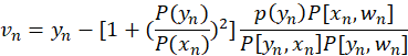
![]()
where P{xn,wn]=![]()
Notice for the Kumar method there is no need to evaluate any derivative of P(x).
Ostrowski's Multi-Point Method
Ostrowski’s multi-point method is:
This method is remarkable since it archived a 4-order convergence rate and only needs to evaluate the P(x) twice and the first derivative P’(x). This yields an efficiency index of 41/3=1.59, better than both the Newton and the Halley methods. The first step is a regular Newton step followed by an enhancement of the step size yielding a 4-order convergence. However, when dealing with multiple roots, it suffers the same fate as the other methods with a linear convergence rate.
What to Do About Multiple Roots
Well, one solution is to realize that the first intermediate step is a classic Newton iteration that has a modified version that can handle multiple roots effectively. Adding the modified Newton step, you get a method to handle multiplicity >1; see below.
Stage 1:

Stage 2:
However, the second refinement does not work well for m> 1. My approach to this is therefore:
- When an iterative step xn is not near a root and we see improvement using the multi-step and or shortening of the step size (see the description of the Newton method), then stick with this modified Newton approach.
- First, when you do not see any improvement using the multi-step check and or shortening of step, then do the second refinement and obtain a 4th-order convergence for the remaining iterations. Well, what about multiplicity greater than one? That is not a problem since it will keep the Newton method at stage 1 and convert quadratic to that root and in that, special case the Ostrowski multi-point method will not be a 4th order method, however for simply root it will, however, be a 4th order method.
How Does the Ostrowski Method Stack Up Against Other Classical Methods?
To see how it works with the different methods, let's see the method against a simple Polynomial.
P(x)= (x-2)(x+2)(x-3)(x+3)=x^4-13x^2+36
The above-mentioned Polynomial is an easy one for most methods. Moreover, as you can see, the higher-order method requires fewer numbers of iterations. However, also more work to be done per iteration.
| Method | Newton | Halley | Household 3rd | Ostrowski |
| Iterations | x | x | x | x |
| Start guess | 0.8320502943378436 | 0.8320502943378436 | 0.8320502943378436 | 0.8320502943378436 |
| 1 | 2.2536991416170737 | 1.6933271400922734 | 2.033435992687734 | 2.0863365344560694 |
| 2 | 1.9233571772166798 | 1.9899385955094577 | 1.9999990577501767 | 1.999968127551831 |
| 3 | 1.9973306906698116 | 1.9999993042509177 | 2 | 2 |
| 4 | 1.999996107736492 | 2 | ||
| 5 | 1.9999999999916678 | |||
| 6 | 2 |
Here is an example of:

The first root ends up as a complex conjugated root x=(1-i) and the third root is another complex conjugated root at (+2-i) and the last root is found directly as x=5. Notice that the search always starts out on the real axis and then rotate into the complex plane after a few iterations.

The above picture shows the convergence rate of approximately 4 for the Ostrowski method while approaching the roots and is in line with expectations.
What to Modify?
Compared to the Newton method (part two) we can luckily reuse most of the code already available with the Newton method.
From Part Two, the steps include:
- Finding an initial point
- Executing the Ostrowski multi-point iteration, including polynomial evaluation via the Horner method
- Calculating the final upper bound
- Polynomial deflation
- Solving the quadratic equation
Ad 1,3,4,5) Will be identical to the Newton method and need no modification
Ad 2) We can simply add the following code to the Stage 2 code after the calculation of the final upper bound to implement the Ostrowski multi-point method.
// Perform the Ostrowski multi-point step
// Pz is P(yn), pzprev is P(zn)
// Do the Ostrowski step as the second part of the multi-point iteration
z = z - pzprev.pz / (pzprev.pz - complex<double>(2) * pz.pz) * pz.pz / p1z.pz;
pz = horner(coeff, z); // Evaluate the new iteration point
The Implementation of the Ostrowski’s Multi-point Method
This is the same source as in parts two and three except for the change needed to evaluate Ostrowski’s multi-point iteration step instead of Newton or Halley.
The implementation of this root finder follows the method as layout in Part One.
- First, we eliminate simple roots (roots equal to zero)
- Then, we find a suitable starting point to start our Newton Iteration, this also includes preliminary termination criteria based on an acceptable value of P(x) where we will stop the current iteration.
- Start the Ostrowski iteration
- The first step is to find the dxn=P(xn)/P’(xn) and of course, decide what should happen if P’(xn) is zero. When this condition arises, it is most often due to a local minimum and the best course of action is to alter the direction with a factor dxn=dxn(0.6+i0.8)m. This is equivalent to rotating the direction with an odd degree of 53 degrees and multiplying the direction with the factor m. A suitable value for m =5 is reasonable when this happens.
- Furthermore, it is easy to realize that if P’(xn)~0. You could get some unreasonable step size of dxn and therefore introduce a limiting factor that reduces the current step size if abs(dxn)>5·abs(dxn-1) than the previous iteration's step size. Again, you alter the direction with dxn=dxn(0.6+i0.8)5(abs(dxn-1)/abs(dxn)).
- These above two modifications make the method very resilient and make it always converge to a root.
- The next issue is to handle the issue with multiplicity > 1 which will slow the 2nd order convergence rate down to a linear convergence rate. After a suitable dxn is found and a new
 , we then look to see if P(xn+1)>P(xn): If so we look at a revised xn+1=xn-0.5dxn and if P(xn+1)≥P(xn) then he used the original xn+1 as the new starting point for the next iteration. If not, then we accept xn+1 as a better choice and continue looking at a newly revised xn+1=xn-0.25dxn. If on the other hand, the new P(xn+1)≥P(xn) we used the previous xn+1 as a new starting point for the next iterations. If not, then we assume we are nearing a new saddle point and the direction is altered with dxn=dxn(0.6+i0.8) and we use xn+1=xn-dxn as the new starting point for the next iteration.
If on the other hand P(xn+1)≤P(xn ): Then we are looking in the right direction and we then continue stepping in that direction using xn+1=xn-mdxn, m=2,..,n as long as P(xn+1)≤P(xn ) and use the best m for the next iterations. The benefit of this process is that if there is a root with the multiplicity of m, then m will also be the best choice for the stepping size and this will maintain the 2nd-order convergence rate even for multiple roots. The last two steps are the same as for the Newton method. - When we get within the convergence circle (stage 2), we bypass step 4 and just add Ostrowski's second step to complete an iteration round.
- Sub processes 1 to 5 continue until the stopping criteria are reached where after the root xn is accepted and deflated up in the Polynomial. A new search for a root using the deflated Polynomial is initiated.
We divide the iterations into two stages. Stage 1 & Stage 2. In stage 1, we are trying to get into the convergence circle where we are sure that Ostrowski’s method will converge towards a root. Since this first step is a regular Newton step, we will use the same computation as the Newton method. When we get into that circle, we automatically switch to stage 2. In stage 2, we skip sub step 4 and just use an unmodified Newton step: followed by Ostrowski's second step: until the stopping criteria have been satisfied. In case we get outside the convergence circle, we switch back to stage 1 and continue the iteration.
We use the same criteria to switch to stage 2 as we did for both the Newton and Halley methods.
Now we have everything we need to determine when to switch to stage 2.
The C++ Code
The C++ code below finds the Polynomial roots with Polynomial real coefficients using Ostrowski’s method. There are only very few changes made from the Newton version to implement Ostrowski’s method. We only added the following few lines of code.
// Perform the Ostrowski multi-point step
// Pz is P(yn), pzprev is P(zn)
// Do the Ostrowski step as the second part of the multi-point iteration
z = z - pzprev.pz / (pzprev.pz - complex<double>(2) * pz.pz) * pz.pz / p1z.pz;
pz = horner(coeff, z); // Evaluate the new iteration point
when switching to stage 2.
Below is the full source.
/*
 *******************************************************************************
 *
 *                       Copyright (c) 2023
 *                       Henrik Vestermark
 *                       Denmark, USA
 *
 *                       All Rights Reserved
 *
 *   This source file is subject to the terms and conditions of
 *   Henrik Vestermark Software License Agreement which restricts the manner
 *   in which it may be used.
 *
 *******************************************************************************
*/

/*
 *******************************************************************************
 *
 * Module name     :   Ostrowski.cpp
 * Module ID Nbr   :
 * Description     :   Solve n degree polynomial using Ostrowski multi-point method
 * --------------------------------------------------------------------------
 * Change Record   :
 *
 * Version    Author/Date        Description of changes
 * -------  -------------    ----------------------
 * 01.01    HVE/24Dec2023    Initial release
 *
 * End of Change Record
 * --------------------------------------------------------------------------
*/

// define version string
static char _VOSTROWSKI_[] = "@(#)testOstrowski.cpp 01.01 -- Copyright (C) Henrik Vestermark";

#include <algorithm>
#include <vector>
#include <complex>
#include <iostream>
#include <functional>

using namespace std;

constexpr int       MAX_ITER = 50;

// Find all polynomial zeros using a modified Newton method
// 1) Eliminate all simple roots (roots equal to zero)
// 2) Find a suitable starting point
// 3) Find a root using Newton
// 4) Divide the root up in the polynomial reducing its order with one
// 5) Repeat steps 2 to 4 until the polynomial is of the order of two
//    whereafter the remaining one or two roots are found by the direct formula
// Notice:
//      The coefficients for p(x) is stored in descending order.
//      coefficients[0] is a(n)x^n, coefficients[1] is a(n-1)x^(n-1),...,
//      coefficients[n-1] is a(1)x, coefficients[n] is a(0)
//
static vector<complex<double>> PolynomialRootsOstrowski(const vector<double>& coefficients)
{
    struct eval { complex<double> z{}; complex<double> pz{}; double apz{}; };
    const complex<double> complexzero(0.0);  // Complex zero (0+i0)
    size_t n;       // Size of Polynomial p(x)
    eval pz;        // P(z)
    eval pzprev;    // P(zprev)
    eval p1z;       // P'(z)
    eval p1zprev;   // P'(zprev)
    complex<double> z;      // Use as temporary variable
    complex<double> dz;     // The current stepsize dz
    int itercnt;    // Hold the number of iterations per root
    vector<complex<double>> roots;  // Holds the roots of the Polynomial
    vector<double> coeff(coefficients.size()); // Holds the current coefficients of P(z)

    copy(coefficients.begin(), coefficients.end(), coeff.begin());
    // Step 1 eliminate all simple roots
    for (n = coeff.size() - 1; n > 0 && coeff.back() == 0.0; --n)
        roots.push_back(complexzero);  // Store zero as the root

    // Compute the next starting point based on the polynomial coefficients
    // A root will always be outside the circle from the origin and radius min
    auto startpoint = [&](const vector<double>& a)
    {
        const size_t n = a.size() - 1;
        double a0 = log(abs(a.back()));
        double min = exp((a0 - log(abs(a.front()))) / static_cast<double>(n));

        for (size_t i = 1; i < n; i++)
            if (a[i] != 0.0)
            {
                double tmp = exp((a0 - log(abs(a[i]))) / static_cast<double>(n - i));
                if (tmp < min)
                    min = tmp;
            }

        return min * 0.5;
    };

    // Evaluate a polynomial with real coefficients a[] at a complex point z and
    // return the result
    // This is Horner's methods avoiding complex arithmetic
    auto horner = [](const vector<double>& a, const complex<double> z)
    {
        const size_t n = a.size() - 1;
        double p = -2.0 * z.real();
        double q = norm(z);
        double s = 0.0;
        double r = a[0];
        eval e;

        for (size_t i = 1; i < n; i++)
        {
            double t = a[i] - p * r - q * s;
            s = r;
            r = t;
        }

        e.z = z;
        e.pz = complex<double>(a[n] + z.real() * r - q * s, z.imag() * r);
        e.apz = abs(e.pz);
        return e;
    };

    // Calculate an upper bound for the rounding errors performed in a
    // polynomial with real coefficient a[] at a complex point z.
    // (Adam's test)
    auto upperbound = [](const vector<double>& a, const complex<double> z)
    {
        const size_t n = a.size() - 1;
        double p = -2.0 * z.real();
        double q = norm(z);
        double u = sqrt(q);
        double s = 0.0;
        double r = a[0];
        double e = fabs(r) * (3.5 / 4.5);
        double t;

        for (size_t i = 1; i < n; i++)
        {
            t = a[i] - p * r - q * s;
            s = r;
            r = t;
            e = u * e + fabs(t);
        }
        t = a[n] + z.real() * r - q * s;
        e = u * e + fabs(t);
        e = (4.5 * e - 3.5 * (fabs(t) + fabs(r) * u) +
            fabs(z.real()) * fabs(r)) * 0.5 * pow((double)_DBL_RADIX, -DBL_MANT_DIG + 1);

        return e;
    };

   // Do Ostrowski iteration for polynomial order higher than 2
    for (; n > 2; --n)
    {
        const double Max_stepsize = 5.0; // Allow the next step size to be up to
                                         // 5 times larger than the previous step size
        const complex<double> rotation = complex<double>(0.6, 0.8);  // Rotation amount
        double r;               // Current radius
        double rprev;           // Previous radius
        double eps;             // The iteration termination value
        bool stage1 = true;     // By default it start the iteration in stage1
        int steps = 1;          // Multisteps if > 1
        vector<double> coeffprime;

        // Calculate coefficients of p'(x)
        for (int i = 0; i < n; i++)
            coeffprime.push_back(coeff[i] * double(n - i));

        // Step 2 find a suitable starting point z
        rprev = startpoint(coeff);      // Computed startpoint
        z = coeff[n - 1] == 0.0 ? complex<double>(1.0) : complex<double>
                            (-coeff[n] / coeff[n - 1]);
        z *= complex<double>(rprev) / abs(z);

        // Setup the iteration
        // Current P(z)
        pz = horner(coeff, z);

        // pzprev which is the previous z or P(0)
        pzprev.z = complex<double>(0);
        pzprev.pz = coeff[n];
        pzprev.apz = abs(pzprev.pz);

        // p1zprev P'(0) is the P'(0)
        p1zprev.z = pzprev.z;
        p1zprev.pz = coeff[n - 1];       // P'(0)
        p1zprev.apz = abs(p1zprev.pz);

        // Set previous dz and calculate the radius of operations.
        dz = pz.z;                 // dz=z-zprev=z since zprev==0
        r = rprev *= Max_stepsize; // Make a reasonable radius of the
                                   // maximum step size allowed
        // Preliminary eps computed at point P(0) by a crude estimation
        eps = 2 * n * pzprev.apz * pow((double)_DBL_RADIX, -DBL_MANT_DIG);

        // Start iteration and stop if z doesnt change or apz <= eps
        // we do z+dz!=z instead of dz!=0. if dz does not change z
        // then we accept z as a root
        for (itercnt = 0; pz.z + dz != pz.z && pz.apz > eps &&
                                 itercnt < MAX_ITER; itercnt++)
        {
     // Calculate current P'(z)
            p1z = horner(coeffprime, pz.z);
            if (p1z.apz == 0.0)                 // P'(z)==0 then rotate and try again
                dz *= rotation * complex<double>(Max_stepsize);  // Multiply with 5
                                                // to get away from saddlepoint
            else
            {
                dz = pz.pz / p1z.pz;  // next dz
                // Check the Magnitude of Newton's step
                r = abs(dz);
                if (r > rprev) // Large than 5 times the previous step size
                {   // then rotate and adjust step size to prevent
                    // wild step size near P'(z) close to zero
                    dz *= rotation * complex<double>(rprev / r);
                    r = abs(dz);
                }
                rprev = r * Max_stepsize;  // Save 5 times the current step size for the
                                           // next iteration check of reasonable step size
                // Calculate if stage1 is true or false. Stage1 is false if the
                // Newton converge otherwise true
                z = (p1zprev.pz - p1z.pz) / (pzprev.z - pz.z);
                stage1 = (abs(z) / p1z.apz > p1z.apz / pz.apz / 4) || (steps != 1);
            }
            // Step accepted. Save pz in pzprev
            pzprev = pz;

            z = pzprev.z - dz;      // Next z
            pz = horner(coeff, z);  //ff = pz.apz;
            // Add this point all we have done is perform a Newton Step
            steps = 1;
            if (stage1)
            {  // Try multiple steps or shorten steps depending if P(z)
               // is an improvement or not P(z)<P(zprev)
                bool div2;
                complex<double> zn;
                eval npz;

                zn = pz.z;
                for (div2 = pz.apz > pzprev.apz; steps <= n; ++steps)
                {
                    if (div2 == true)
                    {  // Shorten steps
                        dz *= complex<double>(0.5);
                        zn = pzprev.z - dz;
                    }
                    else
                        zn -= dz;  // try another step in the same direction

                    // Evaluate new try step
                    npz = horner(coeff, zn);
                    if (npz.apz >= pz.apz)
                        break; // Break if no improvement

                    // Improved => accept step and try another round of step
                    pz = npz;

                    if (div2 == true && steps == 2)
                    {   // To many shorten steps => try another direction and break
                        dz *= rotation;
                        z = pzprev.z - dz;
                        pz = horner(coeff, z);
                        break;
                    }
                }
            }
            else
            {   // calculate the upper bound of error using Adam's test
                // for real coefficients
                // Now that we are within the convergence circle.
                eps = upperbound(coeff, pz.z);
                // Perform the Ostrowski multi-point step
                // Pz is P(yn), pzprev is P(zn)
                // Do the Ostrowski step as the second part of the multi-point iteration
                z = z - pzprev.pz /
                        (pzprev.pz - complex<double>(2) * pz.pz) * pz.pz / p1z.pz;
                pz = horner(coeff, z); // Evaluate the new iteration point
            }
        }

        // Real root forward deflation.
        //
        auto realdeflation = [&](vector<double>& a, const double x)
        {
            const size_t n = a.size() - 1;
            double r = 0.0;

            for (size_t i = 0; i < n; i++)
                a[i] = r = r * x + a[i];

            a.resize(n);    // Remove the highest degree coefficients.
        };

        // Complex root forward deflation for real coefficients
        //
        auto complexdeflation = [&](vector<double>& a, const complex<double> z)
        {
            const size_t n = a.size() - 1;
            double r = -2.0 * z.real();
            double u = norm(z);

            a[1] -= r * a[0];
            for (int i = 2; i < n - 1; i++)
                a[i] = a[i] - r * a[i - 1] - u * a[i - 2];

            a.resize(n - 1); // Remove top 2 highest degree coefficients
        };

        // Check if there is a very small residue in the imaginary part by trying
        // to evaluate P(z.real). if that is less than P(z).
        // We take that z.real() is a better root than z.
        z = complex<double>(pz.z.real(), 0.0);
        pzprev = horner(coeff, z);
        if (pzprev.apz <= pz.apz)
        { // real root
            pz = pzprev;
            // Save the root
            roots.push_back(pz.z);
            realdeflation(coeff, pz.z.real());
        }
        else
        {   // Complex root
            // Save the root
            roots.push_back(pz.z);
            roots.push_back(conj(pz.z));
            complexdeflation(coeff, pz.z);
            --n;
        }

    }   // End Iteration

    // Solve any remaining linear or quadratic polynomial
    // For Polynomial with real coefficients a[],
    // The complex solutions are stored in the back of the roots
    auto quadratic = [&](const std::vector<double>& a)
    {
        const size_t n = a.size() - 1;
        complex<double> v;
        double r;

        // Notice that a[0] is !=0 since roots=zero has already been handle
        if (n == 1)
            roots.push_back(complex<double>(-a[1] / a[0], 0));
        else
        {
            if (a[1] == 0.0)
            {
                r = -a[2] / a[0];
                if (r < 0)
                {
                    r = sqrt(-r);
                    v = complex<double>(0, r);
                    roots.push_back(v);
                    roots.push_back(conj(v));
                }
                else
                {
                    r = sqrt(r);
                    roots.push_back(complex<double>(r));
                    roots.push_back(complex<double>(-r));
                }
            }
            else
            {
                r = 1.0 - 4.0 * a[0] * a[2] / (a[1] * a[1]);
                if (r < 0)
                {
                    v = complex<double>(-a[1] / (2.0 * a[0]),
                                         a[1] * sqrt(-r) / (2.0 * a[0]));
                    roots.push_back(v);
                    roots.push_back(conj(v));
                }
                else
                {
                    v = complex<double>((-1.0 - sqrt(r)) * a[1] / (2.0 * a[0]));
                    roots.push_back(v);
                    v = complex<double>(a[2] / (a[0] * v.real()));
                    roots.push_back(v);
                }
            }
        }
        return;
    };

    if (n > 0)
        quadratic(coeff);

    return roots;
}
Example 1
Here is an example of how the above source code is working.
For the real Polynomial:
+1x^4-10x^3+35x^2-50x+24
Start Ostrowski Iteration for Polynomial=+1x^4-10x^3+35x^2-50x+24
Stage 1=>Stop Condition. |f(z)|<2.13e-14
Start: z[1]=0.2 dz=2.40e-1 |f(z)|=1.4e+1
Iteration: 1
Ostrowski Step: z[1]=0.6 dz=-3.98e-1 |f(z)|=3.9e+0
Function value decrease=>try multiple steps in that direction
Try Step: z[1]=1 dz=-3.98e-1 |f(z)|=2.0e-1
: Improved. Continue stepping
Try Step: z[1]=1 dz=-3.98e-1 |f(z)|=9.9e-1
: No improvement. Discard the last try step
Iteration: 2
Ostrowski Step: z[1]=1 dz=3.87e-2 |f(z)|=1.6e-2
Function value decrease=>try multiple steps in that direction
Try Step: z[1]=1 dz=3.87e-2 |f(z)|=2.7e-1
: No improvement. Discard the last try step
Ostrowski Stage 2 Step: z[1]=1 dz=-2.63e-3 |f(z)|=5.3e-5
Iteration: 3
Ostrowski Step: z[1]=1 dz=-8.78e-6 |f(z)|=8.5e-10
In Stage 2. New Stop Condition: |f(z)|<2.18e-14
Ostrowski Stage 2 Step: z[1]=1 dz=-1.41e-10 |f(z)|=0
Stop Criteria satisfied after 3 Iterations
Final Ostrowski z[1]=1 dz=-8.78e-6 |f(z)|=0
Alteration=0% Stage 1=67% Stage 2=33%
Deflate the real root z=1
Start Ostrowski Iteration for Polynomial=+1x^3-9x^2+26x-24
Stage 1=>Stop Condition. |f(z)|<1.60e-14
Start : z[1]=0.5 dz=4.62e-1 |f(z)|=1.4e+1
Iteration: 1
Ostrowski Step: z[1]=1 dz=-7.54e-1 |f(z)|=3.9e+0
Function value decrease=>try multiple steps in that direction
Try Step: z[1]=2 dz=-7.54e-1 |f(z)|=6.4e-2
: Improved. Continue stepping
Try Step: z[1]=3 dz=-7.54e-1 |f(z)|=2.6e-1
: No improvement. Discard the last try step
Iteration: 2
Ostrowski Step: z[1]=2 dz=-2.95e-2 |f(z)|=2.7e-3
Function value decrease=>try multiple steps in that direction
Try Step: z[1]=2 dz=-2.95e-2 |f(z)|=5.4e-2
: No improvement. Discard the last try step
Ostrowski Stage 2 Step: z[1]=2 dz=-1.32e-3 |f(z)|=4.1e-6
Iteration: 3
Ostrowski Step: z[1]=2 dz=-2.06e-6 |f(z)|=1.3e-11
In Stage 2. New Stop Condition: |f(z)|<1.42e-14
Ostrowski Stage 2 Step: z[1]=2 dz=-6.36e-12 |f(z)|=0
Stop Criteria satisfied after 3 Iterations
Final Ostrowski z[1]=2 dz=-2.06e-6 |f(z)|=0
Alteration=0% Stage 1=67% Stage 2=33%
Deflate the real root z=2.0000000000000004
Solve Polynomial=+1x^2-7x+11.999999999999996 directly
Using the Ostrowski Method, the Solutions are:
X1=1
X2=2.0000000000000004
X3=4.000000000000003
X4=2.9999999999999973
Time used: 0 msec. Solvable level: Easy

Example 2
The same example just with a double root at x=1. We see that each step is a double step in line with a multiplicity of 2 for the first root.
For the real Polynomial:
+1x^4-9x^3+27x^2-31x+12
Start Ostrowski Iteration for Polynomial=+1x^4-9x^3+27x^2-31x+12
Stage 1=>Stop Condition. |f(z)|<1.07e-14
Start : z[1]=0.2 dz=1.94e-1 |f(z)|=6.9e+0
Iteration: 1
Ostrowski Step: z[1]=0.5 dz=-3.23e-1 |f(z)|=2.0e+0
Function value decrease=>try multiple steps in that direction
Try Step: z[1]=0.8 dz=-3.23e-1 |f(z)|=1.8e-1
: Improved. Continue stepping
Try Step: z[1]=1 dz=-3.23e-1 |f(z)|=1.4e-1
: Improved. Continue stepping
Try Step: z[1]=1 dz=-3.23e-1 |f(z)|=8.9e-1
: No improvement. Discard the last try step
Iteration: 2
Ostrowski Step: z[1]=1 dz=8.71e-2 |f(z)|=3.1e-2
Function value decrease=>try multiple steps in that direction
Try Step: z[1]=1 dz=8.71e-2 |f(z)|=9.6e-4
: Improved. Continue stepping
Try Step: z[1]=0.9 dz=8.71e-2 |f(z)|=6.5e-2
: No improvement. Discard the last try step
Iteration: 3
Ostrowski Step: z[1]=1 dz=-6.27e-3 |f(z)|=2.4e-4
Function value decrease=>try multiple steps in that direction
Try Step: z[1]=1 dz=-6.27e-3 |f(z)|=2.6e-8
: Improved. Continue stepping
Try Step: z[1]=1 dz=-6.27e-3 |f(z)|=2.3e-4
: No improvement. Discard the last try step
Iteration: 4
Ostrowski Step: z[1]=1 dz=-3.28e-5 |f(z)|=6.5e-9
Function value decrease=>try multiple steps in that direction
Try Step: z[1]=1 dz=-3.28e-5 |f(z)|=0
: Improved. Continue stepping
Try Step: z[1]=1 dz=-3.28e-5 |f(z)|=6.5e-9
: No improvement. Discard the last try step
Stop Criteria satisfied after 4 Iterations
Final Ostrowski z[1]=1 dz=-3.28e-5 |f(z)|=0
Alteration=0% Stage 1=100% Stage 2=0%
Deflate the real root z=0.9999999982094424
Start Ostrowski Iteration for Polynomial=+1x^3-8.000000001790557x^2+19.000000012533903x-12.000000021486692
Stage 1=>Stop Condition. |f(z)|<7.99e-15
Start : z[1]=0.3 dz=3.16e-1 |f(z)|=6.8e+0
Iteration: 1
Ostrowski Step: z[1]=0.8 dz=-4.75e-1 |f(z)|=1.5e+0
Function value decrease=>try multiple steps in that direction
Try Step: z[1]=1 dz=-4.75e-1 |f(z)|=1.3e+0
: Improved. Continue stepping
Try Step: z[1]=2 dz=-4.75e-1 |f(z)|=2.1e+0
: No improvement. Discard the last try step
Iteration: 2
Ostrowski Step: z[1]=0.9 dz=3.54e-1 |f(z)|=5.7e-1
Function value decrease=>try multiple steps in that direction
Try Step: z[1]=0.6 dz=3.54e-1 |f(z)|=3.7e+0
: No improvement. Discard the last try step
Ostrowski Stage 2 Step: z[1]=1 dz=-8.44e-2 |f(z)|=2.6e-2
Iteration: 3
Ostrowski Step: z[1]=1 dz=-4.35e-3 |f(z)|=9.5e-5
In Stage 2. New Stop Condition: |f(z)|<6.66e-15
Ostrowski Stage 2 Step: z[1]=1 dz=-1.58e-5 |f(z)|=9.5e-10
Iteration: 4
Ostrowski Step: z[1]=1 dz=-1.58e-10 |f(z)|=8.9e-16
In Stage 2. New Stop Condition: |f(z)|<6.66e-15
Ostrowski Stage 2 Step: z[1]=1 dz=1.48e-16 |f(z)|=8.9e-16
Stop Criteria satisfied after 4 Iterations
Final Ostrowski z[1]=1 dz=-1.58e-10 |f(z)|=8.9e-16
Alteration=0% Stage 1=50% Stage 2=50%
Deflate the real root z=1.0000000017905575
Solve Polynomial=+1x^2-7x+12 directly
Using the Ostrowski Method, the Solutions are:
X1=0.9999999982094424
X2=1.0000000017905575
X3=4
X4=3
Time used: 1 msec. Solvable level: Easy

Example 3
A test polynomial with both real and complex conjugated roots.
For the real Polynomial:
+1x^4-8x^3-17x^2-26x-40
Start Ostrowski Iteration for Polynomial=+1x^4-8x^3-17x^2-26x-40
Stage 1=>Stop Condition. |f(z)|<3.55e-14
Start : z[1]=-0.8 dz=-7.67e-1 |f(z)|=2.6e+1
Iteration: 1
Ostrowski Step: z[1]=-2 dz=1.65e+0 |f(z)|=7.0e+1
Function value increase=>try shorten the step
Try Step: z[1]=-2 dz=8.24e-1 |f(z)|=3.1e+0
: Improved=>Continue stepping
Try Step: z[1]=-1 dz=4.12e-1 |f(z)|=1.8e+1
: No improvement=>Discard last try step
Iteration: 2
Ostrowski Step: z[1]=-2 dz=6.27e-2 |f(z)|=1.5e-1
Function value decrease=>try multiple steps in that direction
Try Step: z[1]=-2 dz=6.27e-2 |f(z)|=3.7e+0
: No improvement. Discard the last try step
Ostrowski Stage 2 Step: z[1]=-2 dz=-2.74e-3 |f(z)|=1.4e-4
Iteration: 3
Ostrowski Step: z[1]=-2 dz=-2.58e-6 |f(z)|=2.6e-10
In Stage 2. New Stop Condition: |f(z)|<1.91e-14
Ostrowski Stage 2 Step: z[1]=-2 dz=-4.88e-12 |f(z)|=0
Stop Criteria satisfied after 3 Iterations
Final Ostrowski z[1]=-2 dz=-2.58e-6 |f(z)|=0
Alteration=0% Stage 1=67% Stage 2=33%
Deflate the real root z=-1.650629191439388
Start Ostrowski Iteration for Polynomial=+1x^3-9.650629191439387x^2-1.0703897408530487x-24.233183447530717
Stage 1=>Stop Condition. |f(z)|<1.61e-14
Start : z[1]=-0.8 dz=-7.92e-1 |f(z)|=3.0e+1
Iteration: 1
Ostrowski Step: z[1]=1 dz=-1.86e+0 |f(z)|=3.5e+1
Function value increase=>try shorten the step
Try Step: z[1]=0.1 dz=-9.30e-1 |f(z)|=2.5e+1
: Improved=>Continue stepping
Try Step: z[1]=-0.3 dz=-4.65e-1 |f(z)|=2.5e+1
: No improvement=>Discard last try step
Iteration: 2
Ostrowski Step: z[1]=-7 dz=6.71e+0 |f(z)|=7.2e+2
Function value increase=>try shorten the step
Try Step: z[1]=-3 dz=3.35e+0 |f(z)|=1.5e+2
: Improved=>Continue stepping
Try Step: z[1]=-2 dz=1.68e+0 |f(z)|=4.9e+1
: Improved=>Continue stepping
: Probably local saddlepoint=>Alter Direction: z[1]=(-0.4-i0.7) dz=(5.03e-1+i6.71e-1) |f(z)|=2.1e+1
Iteration: 3
Ostrowski Step: z[1]=(0.3-i2) dz=(-6.86e-1+i1.17e+0) |f(z)|=1.9e+1
Function value decrease=>try multiple steps in that direction
Try Step: z[1]=(1-i3) dz=(-6.86e-1+i1.17e+0) |f(z)|=8.4e+1
: No improvement. Discard the last try step
Ostrowski Stage 2 Step: z[1]=(-0.09-i2) dz=(4.13e-1-i3.17e-1) |f(z)|=2.6e+0
Iteration: 4
Ostrowski Step: z[2]=(-0.18-i1.5) dz=(8.33e-2+i2.00e-2) |f(z)|=8.1e-2
In Stage 2. New Stop Condition: |f(z)|<1.36e-14
Ostrowski Stage 2 Step: z[4]=(-0.1747-i1.547) dz=(-1.74e-3+i1.86e-3) |f(z)|=6.2e-5
Iteration: 5
Ostrowski Step: z[7]=(-0.1746854-i1.546869) dz=(1.94e-6-i4.50e-8) |f(z)|=4.2e-11
In Stage 2. New Stop Condition: |f(z)|<1.36e-14
Ostrowski Stage 2 Step: z[13]=(-0.1746854042803-i1.546868887231) dz=(-3.03e-13+i1.29e-12) |f(z)|=3.6e-15
Stop Criteria satisfied after 5 Iterations
Final Ostrowski z[7]=(-0.1746854-i1.546869) dz=(1.94e-6-i4.50e-8) |f(z)|=3.6e-15
Alteration=20% Stage 1=60% Stage 2=40%
Deflate the complex conjugated root z=(-0.17468540428030602-i1.546868887231396)
Solve Polynomial=+1x-10 directly
Using the Ostrowski Method, the Solutions are:
X1=-1.650629191439388
X2=(-0.17468540428030602-i1.546868887231396)
X3=(-0.17468540428030602+i1.546868887231396)
X4=10
Time used: 1 msec. Solvable level: Easy


The iterations trail towards the first two roots.
Recommendation
Since the efficiency index is higher than Newton, Halley, and others methods, Ostrowski’s multi-point is worth considering. However, there is one notorious flaw and that is the reduction in convergence order when encountering multiple roots. Since you can still maintain a convergence order of 2 in these cases, you could consider it better than the Newton method due to its higher efficiency index of 1.59 (compared to 1.41 Newton) when dealing with well-separated roots.
Final Remarks
In this series of papers, we have addressed many of the classical methods, e.g., fixed point, multi-point, simultaneous methods, etc. However, I have omitted two methods that are also worth mentioning and that is the famous “black-box” method by Jenkins-Traub and of course, the eigenvalue method. Both of these methods are worth a separate paper maybe for a further expansion of this paper series. Nevertheless, despite being quite different methods explained in the sixth installment, all of them can be wrapped into the same framework as established in part one and two and going from one method to another, you only need to change a few lines of code here and there while still maintain the robustness, resiliency, and efficient implementation of each method.
A web-based polynomial solver showcasing these various methods is available for further exploration and can be found on Polynomial roots (http://hvks.com/Numerical/websolver.php) that demonstrate all of these methods in action.
References
- H. Vestermark. A practical implementation of Polynomial root finders. Practical implementation of Polynomial root finders vs 7.docx (www.hvks.com)
- Madsen. A root-finding algorithm based on Newton Method, Bit 13 (1973) 71-75.
- A. Ostrowski, Solution of equations and systems of equations, Academic Press, 1966.
- Wikipedia Horner’s Method: https://en.wikipedia.org/wiki/Horner%27s_method
- Adams, D A stopping criterion for polynomial root finding. Communication of the ACM Volume 10/Number 10/ October 1967 Page 655-658
- Grant, J. A. & Hitchins, G D. Two algorithms for the solution of polynomial equations to limiting machine precision. The Computer Journal Volume 18 Number 3, pages 258-264
- Wilkinson, J H, Rounding errors in Algebraic Processes, Prentice-Hall Inc, Englewood Cliffs, NJ 1963
- McNamee, J.M., Numerical Methods for Roots of Polynomials, Part I & II, Elsevier, Kidlington, Oxford 2009
- H. Vestermark, “A Modified Newton and higher orders Iteration for multiple roots.”, www.hvks.com/Numerical/papers.html
- M.A. Jenkins & J.F. Traub, ”A three-stage Algorithm for Real Polynomials using Quadratic iteration”, SIAM J Numerical Analysis, Vol. 7, No.4, December 1970.
History
- 8th January, 2024: Some images were missing from the original submission
- 6th January, 2024: Initial version of Ostrowski's multi-point method