
Fast and Stable Polynomial Root Finders - Part Three
5.00/5 (7 votes)
Practical implementation of a fast, robust and stable polynomial root finder using Halley's method
Contents
- Introduction
- Higher order method
- Comparing Newton and Halley
- What to Modify?
- The Implementation of the Halley Algorithm
- The C++ code
- Householder 3rd order method
- How the higher orders method stacks up against each other
- Other Higher order method
- Recommendation
- Conclusion
- References
- History
Introduction
In the first paper (Part One), we developed a highly efficient and robust polynomial root-finder based on the Newton method, specifically designed for complex polynomial coefficients. In Part Two, we elaborated on the change to dealing with Polynomials with real coefficients. In Part Three, we look at using the same framework to implement higher-order methods and discuss if we gain any advantages from using higher-order methods compared to the standard Newton method.
Higher Order Method
The Newton method has a convergence rate of two meaning that for every iteration, you double the number of correct digits. However, there exist other higher-order methods that have a convergence rate of 3, 4, 5 6, or even higher. One of them is the Halley method which has a convergence rate of three (or cubic). The cubic convergence rate indicates that we triple the correct number of digits per iteration. The Halley method uses an iteration based on the following recurrence:

Compared to our modified Newton:

We need to evaluate the second derivate of P(x) and do some extra arithmetic operations.
The Halley method is sometimes written as:

Where ![]() is the usual Newton iteration multiplied with the Halley correction:
is the usual Newton iteration multiplied with the Halley correction:

And are graphically shown below:

As for the Newton method, we don’t use this version since it will show the same weakness as the original Newton step when dealing with roots with a multiplicity higher than 1 (multiple roots).
In [8], they present a formula for multiple roots, where m is the multiplicity of the root:

Since m represents the multiplicity of the root. It changes the Halley adjustment based on m, you would have to recalculate the Halley adjustment for each m.
Below is an alternative slightly different modified version of the Halley method that also maintains the cubic convergence rate even for multiple roots but where m is placed outside making it easier to calculate since the Halley adjustment is unchanged.

Alternatively, it is written in another way:

Both formulas will work and maintain cubic convergence.
Here is an example:

For the first root x1~ -1.65, we start at ~ -0.8 and iterate along the real axis towards the root at ~ -1.65. Since we never leave the real axis, we don’t have to see a miniscule imaginary part in the result. The first root is deflated and we start a new search with the deflated polynomial x3-9.650629191439387x2-1.0703897408530487x-24.233183447530717. We again start out on the real axis around ~ -0.8, but this time we are near a saddle point and rotate into the complex plane. After 5 iterations, we find the complex root ~(-0.17-i1.54). We deflate the polynomial with its complex and complex conjugated root and end up with a first-degree polynomial that we solved direct and get x=10.
Comparing Newton and Halley
To compare different methods with others, we can use a well-known efficiency index to see how it stacks up against other derivative-based methods.
The efficiency index is q(1/p), where q is the method convergence order and p are the number of polynomial evaluations for the method. For the Newton, method p is 2 since we need to evaluate both P(z) and P’(z) per iteration, and the Newton method has a convergence order of q=2 so we get Efficiency index= 2(1/2)=1.42
For the Halley method, we need to evaluate P(x), P’(x), and P’’(x) for each iteration, we get 3(1/3)=1.44
Slightly larger than the Newton method but not enough that we should expect any measurable gain from using the Halley method.
What to Modify?
Compared to the Newton method (Part Two), we can luckily reuse most of the code already available with the Newton method.
From Part Two, the steps include:
- Finding an initial point
- Executing the Newton iteration, including polynomial evaluation via the Horner method
- Calculating the final upper bound
- Polynomial deflation
- Solving the quadratic equation
Ad 1,3,4,5) Will be identical and need no modification
Ad 2) We can use the Horned method unchanged to evaluate P(x), P’(x), and P’’(x). Although we need to add another vector to hold the second derivative of P(x). The variable step size to handle multiple roots can be changed from m to (m+1)/2m. Otherwise, we can again reuse the variable step size or reduce the step size and show it in both parts one and two.
The Implementation of the Halley Algorithm
This is the same source as in Part Two except for the change needed to evaluate the second derivative and perform the Halley step instead of the Newton step.
The implementation of this root finder follows the method as layout in Part One.
- First, we eliminate simple roots (roots equal to zero)
- Then, we find a suitable starting point to start our Halley Iteration, this also includes termination criteria based on an acceptable value of P(x) where we will stop the current iteration.
- Start the Halley iteration
- The first step is to find the dxn=
 and of course, decide what should happen if P’(xn) is zero. When this condition arises, it is most often due to a local minimum and the best course of action is to alter the direction with a factor dxn=dxn(0.6+i0.8)k. This is equivalent to rotating the direction with an odd degree of 53 degrees and multiplying the direction with the factor k. A suitable value for k=5 is reasonable when this happens.
 - Furthermore, it is easy to realize that if P’(xn)~0. You could get some unreasonable step size of dxn and therefore introduce a limiting factor that reduces the current step size if abs(dxn)>5·abs(dxn-1) than the previous iteration's step size. Again, you alter the direction with dxn=dxn(0.6+i0.8)5(abs(dxn-1)/abs(dxn)) if that happens.
- These two modifications (a and b) make his method very resilient and make it always converge to a root.
- The next issue is to handle the issue with multiplicity > 1 which will slow the third-order convergence rate down to a linear convergence rate. After a suitable dxn is found and a new xn+1=xn-dxn we then look to see if P(xn+1)>P(xn): If so we look at a revised xn+1=xn-0.5dxn and if P(xn+1)≥P(xn) then he used the original xn+1 as the new starting point for the next iteration. If not then we accept xn+1 as a better choice and continue looking at a newly revised xn+1=xn-0.25dxn. If on the other hand, the new P(xn+1)≥P(xn) we used the previous xn+1 as a new starting point for the next iterations. If not, then we assume we are nearing a new saddle point and the direction is altered with dxn=dxn(0.6+i0.8) and we use xn+1=xn-dxn as the new starting point for the next iteration.
if on the other hand P(xn+1)≤P(xn): Then we are looking in the right direction and we then continue stepping in that direction using:
 m=2,..,n as long as P(xn+1)≤P(xn) and use the best m for the next iterations. The benefit of this process is that if there is a root with the multiplicity of m, then m will also be the best choice for the stepping size and this will maintain the third-order convergence rate even for multiple roots.
 - The first step is to find the dxn=
- Processes a-d continue until the stopping criteria are reached where after the root xn is accepted and deflated up in the Polynomial. A new search for a root using the deflated Polynomial is initiated.
In [2], they divide the iterations into two stages. Stage 1 & Stage 2. In Stage 1, we are trying to get into the convergence circle where we are sure that the Halley method will converge towards a root. When we get into that circle, we automatically switch to stage 2. In Stage 2, we skip step d) and just use an unmodified Halley step:  until the stopping criteria have been satisfied. In case we get outside the convergence circle, we switch back to stage 1 and continue the iteration.
In [2], they use the following criteria to switch to stage 2 based on the theorem 7.1 from Ostrowski [3] that states if K is a circle with center w-P(w)/P'(w) And radius |P(w)/P'(w)|
Then we have guarantee convergence if the following two conditions are satisfied:
![]()

Although this is originally the check for Newton convergence, we use it also for the Halley iterations with initial value w will lead to a convergence of zero within the circle K. To simplify the calculation, we make 2 substitutes, since ![]() and instead of p”(w), we replace it with a difference approximation
and instead of p”(w), we replace it with a difference approximation ![]()
Now we have everything we need to determine when to switch to stage 2.
The C++ Code
The C++ code below finds the Polynomial roots with Polynomial real coefficients using the Halley method. There are only very few changes made to the Newton version to implement the Halley method. The few lines of code are all marked with a comment // Halley. See [1] for details.
/*
 *******************************************************************************
 *
 *                       Copyright (c) 2023
 *                       Henrik Vestermark
 *                       Denmark, USA
 *
 *                       All Rights Reserved
 *
 *   This source file is subject to the terms and conditions of
 *   Henrik Vestermark Software License Agreement which restricts the manner
 *   in which it may be used.
 *
 *******************************************************************************
*/
/*
 *******************************************************************************
 *
 * Module name     :   Halley.cpp
 * Module ID Nbr   :
 * Description     :   Solve n degree polynomial using Halley's method
 * --------------------------------------------------------------------------
 * Change Record   :
 *
 * Version Author/Date Description of changes
 * -------  ------------- ----------------------
 * 01.01 HVE/24Sep2023 Initial release
 *
 * End of Change Record
 * --------------------------------------------------------------------------
*/

// define version string
static char _VHALLEY_[] = "@(#)testHalley.cpp 01.01 -- Copyright (C) Henrik Vestermark";
#include <algorithm>
#include <vector>
#include <complex>
#include <iostream>
#include <functional>

using namespace std;
constexpr int       MAX_ITER = 50;

// Find all polynomial zeros using a modified Halley method
// 1) Eliminate all simple roots (roots equal to zero)
// 2) Find a suitable starting point
// 3) Find a root using the Halley method
// 4) Divide the root up in the polynomial reducing its order with one
// 5) Repeat steps 2 to 4 until the polynomial is of the order of two
// whereafter the remaining one or two roots are found by the direct formula
// Notice:
//      The coefficients for p(x) is stored in descending order.
//      coefficients[0] is a(n)x^n, coefficients[1] is a(n-1)x^(n-1),...,
//      coefficients[n-1] is a(1)x, coefficients[n] is a(0)
//
static vector<complex<double>> PolynomialRootsHalley(const vector<double>& coefficients)
{
    struct eval { complex<double> z{}; complex<double> pz{}; double apz{}; };
    const complex<double> complexzero(0.0);  // Complex zero (0+i0)
    size_t n;       // Size of Polynomial p(x)
    eval pz;        // P(z)
    eval pzprev;    // P(zprev)
    eval p1z;       // P'(z)
    eval p1zprev;   // P'(zprev)
    complex<double> z;      // Use as temporary variable
    complex<double> dz;     // The current stepsize dz
    int itercnt;    // Hold the number of iterations per root
    vector<complex<double>> roots;  // Holds the roots of the Polynomial
    vector<double> coeff(coefficients.size()); // Holds the current coefficients of P(z)

    copy(coefficients.begin(), coefficients.end(), coeff.begin());
    // Step 1 eliminate all simple roots
    for (n = coeff.size() - 1; n > 0 && coeff.back() == 0.0; --n)
        roots.push_back(complexzero);  // Store zero as the root

    // Compute the next starting point based on the polynomial coefficients
    // A root will always be outside the circle from the origin and radius min
    auto startpoint = [&](const vector<double>& a)
    {
        const size_t n = a.size() - 1;
        double a0 = log(abs(a.back()));
        double min = exp((a0 - log(abs(a.front()))) / static_cast<double>(n));

        for (size_t i = 1; i < n; i++)
            if (a[i] != 0.0)
            {
                double tmp = exp((a0 - log(abs(a[i]))) / static_cast<double>(n - i));
                if (tmp < min)
                    min = tmp;
            }

        return min * 0.5;
    };

    // Evaluate a polynomial with real coefficients a[] at a complex point z and
    // return the result
    // This is Horner's methods avoiding complex arithmetic
    auto horner = [](const vector<double>& a, const complex<double> z)
    {
        const size_t n = a.size() - 1;
        double p = -2.0 * z.real();
        double q = norm(z);
        double s = 0.0;
        double r = a[0];
        eval e;

        for (size_t i = 1; i < n; i++)
        {
            double t = a[i] - p * r - q * s;
            s = r;
            r = t;
        }

        e.z = z;
        e.pz = complex<double>(a[n] + z.real() * r - q * s, z.imag() * r);
        e.apz = abs(e.pz);
        return e;
    };

    // Calculate an upper bound for the rounding errors performed in a
    // polynomial with real coefficient a[] at a complex point z.
    // (Adam's test)
    auto upperbound = [](const vector<double>& a, const complex<double> z)
    {
        const size_t n = a.size() - 1;
        double p = -2.0 * z.real();
        double q = norm(z);
        double u = sqrt(q);
        double s = 0.0;
        double r = a[0];
        double e = fabs(r) * (3.5 / 4.5);
        double t;

        for (size_t i = 1; i < n; i++)
        {
            t = a[i] - p * r - q * s;
            s = r;
            r = t;
            e = u * e + fabs(t);
        }

        t = a[n] + z.real() * r - q * s;
        e = u * e + fabs(t);
        e = (4.5 * e - 3.5 * (fabs(t) + fabs(r) * u) +
            fabs(z.real()) * fabs(r)) * 0.5 * pow((double)_DBL_RADIX, -DBL_MANT_DIG + 1);

        return e;
    };

    // Do Newton iteration for polynomial order higher than 2
    for (; n > 2; --n)
    {
        const double Max_stepsize = 5.0; // Allow the next step size to be
                               // up to 5 times larger than the previous step size
        const complex<double> rotation = complex<double>(0.6, 0.8);  // Rotation amount
        double r;              // Current radius
        double rprev;          // Previous radius
        double eps;            // The iteration termination value
        bool stage1 = true;    // By default it start the iteration in stage1
        int steps = 1;         // Multisteps if > 1
        eval p2z;              // P''(z)
        vector<double> coeffprime;   // vector holding the prime coefficients
        vector<double> coeffprime2;  // Halley vector holding both the
                                           // prime and double prime coefficients

        // Calculate coefficients of p'(x)
        for (int i = 0; i < n; i++)
            coeffprime.push_back(coeff[i] * double(n - i));

        // Calculate coefficients of p''(x)
        for (int i = 0; i < n-1; i++)       // Halley
            coeffprime2.push_back(coeffprime[i] * double(n-i-1));   // Halley

        // Step 2 find a suitable starting point z
        rprev = startpoint(coeff);             // Computed startpoint
        z = coeff[n - 1] == 0.0 ? complex<double>(1.0) :
            complex<double>(-coeff[n] / coeff[n - 1]);
        z *= complex<double>(rprev) / abs(z);

        // Setup the iteration
        // Current P(z)
        pz = horner(coeff, z);

        // pzprev which is the previous z or P(0)
        pzprev.z = complex<double>(0);
        pzprev.pz = coeff[n];
        pzprev.apz = abs(pzprev.pz);

        // p1zprev P'(0) is the P'(0)
        p1zprev.z = pzprev.z;
        p1zprev.pz = coeff[n - 1];       // P'(0)
        p1zprev.apz = abs(p1zprev.pz);

        // Set previous dz and calculate the radius of operations.
        dz = pz.z;                 // dz=z-zprev=z since zprev==0
        r = rprev *= Max_stepsize; // Make a reasonable radius
                                   // of the maximum step size allowed
        // Preliminary eps computed at point P(0) by a crude estimation
        eps = 4 * n * pzprev.apz * pow((double)_DBL_RADIX, -DBL_MANT_DIG);

        // Start iteration and stop if z doesn't change or apz <= eps
        // we do z+dz!=z instead of dz!=0. if dz does not change z
        // then we accept z as a root
        for (itercnt = 0; pz.z + dz != pz.z && pz.apz >
             eps && itercnt < MAX_ITER; itercnt++)
        {
            complex<double> halleyfactor;
            complex<double> newtondz;
            // Calculate current P'(z)
            p1z = horner(coeffprime, pz.z);
            if (p1z.apz == 0.0)                 // P'(z)==0 then rotate and try again
                dz *= rotation * complex<double>(Max_stepsize);  // Multiply with 5
                                                // to get away from saddlepoint
            else
            {
                dz = pz.pz / p1z.pz;  // next Newton step dz
                // Calculate hte Halley factor
                // Calculate current P''(z)
                p2z = horner(coeffprime2, pz.z);        // Halley
                // Calculate the Halley factor
                halleyfactor = complex<double>(1.0) -
                     complex<double>(0.5) * dz * (p2z.pz / p1z.pz); // Halley
                newtondz = dz;              // Halley. Save Newton step size
                dz /= halleyfactor;         // Halley step size

                // Check the Magnitude of Halley's step
                r = abs(dz);
                if (r > rprev) // Large than 5 times the previous step size
                {   // then rotate and adjust step size to prevent
                    // wild step size near P'(z) close to zero
                    dz *= rotation * complex<double>(rprev / r);
                    r = abs(dz);
                }

                rprev = r * Max_stepsize;  // Save 5 times the current step size
                                           // for the next iteration check of
                                           // reasonable step size

                // Calculate if stage1 is true or false.
                // Stage1 is false if the Newton/Halley converge otherwise true
                z = (p1zprev.pz - p1z.pz) / (pzprev.z - pz.z);
                stage1 = (abs(z) / p1z.apz > p1z.apz / pz.apz / 4) || (steps != 1);
            }

            // Step accepted. Save pz in pzprev
            pzprev = pz;

            z = pzprev.z - dz;      // Next z
            pz = horner(coeff, z); //ff = pz.apz;
            steps = 1;

            if (stage1)
            {  // Try multiple steps or shorten steps depending if
               // P(z) is an improvement or not P(z)<P(zprev)
                bool div2;
                complex<double> zn, dzn=dz;
                eval npz;

                zn = pz.z;
                steps++;
                for (div2 = pz.apz > pzprev.apz; steps <= n; ++steps)
                {
                    if (div2 == true)
                    {  // Shorten steps
                        dz *= complex<double>(0.5);
                        zn = pzprev.z - dz;
                    }
                    else
                    {
                        halleyfactor = complex<double>((steps+1.0)/(2.0*steps)) -
                            complex<double>(0.5) * newtondz * p2z.pz / p1z.pz; // Halley
                        zn = pzprev.z - newtondz / halleyfactor;  // Halley try
                                                 // another step in the same direction
                    }

                    // Evaluate new try step
                    npz = horner(coeff, zn);
                    if (npz.apz >= pz.apz)
                    {
                        --steps; break; // Break if no improvement
                    }

                    // Improved => accept step and try another round of step
                    pz = npz;
                    dz = dzn;

                    if (div2 == true && steps == 3)
                    {   // To many shorten steps => try another direction and break
                        dz *= rotation;
                        z = pzprev.z - dz;
                        pz = horner(coeff, z);
                        break;
                    }
                }
            }
            else
            {   // calculate the upper bound of error using
                // Grant & Hitchins's test for complex coefficients
                // Now that we are within the convergence circle.
                eps = upperbound(coeff, pz.z);
            }
        }

        // Real root forward deflation.
        //
        auto realdeflation = [&](vector<double>& a, const double x)
        {
            const size_t n = a.size() - 1;
            double r = 0.0;

            for (size_t i = 0; i < n; i++)
                a[i] = r = r * x + a[i];

            a.resize(n);    // Remove the highest degree coefficients.
        };

        // Complex root forward deflation for real coefficients
        //
        auto complexdeflation = [&](vector<double>& a, const complex<double> z)
        {
            const size_t n = a.size() - 1;
            double r = -2.0 * z.real();
            double u = norm(z);

            a[1] -= r * a[0];
            for (int i = 2; i < n - 1; i++)
                a[i] = a[i] - r * a[i - 1] - u * a[i - 2];

            a.resize(n - 1); // Remove top 2 highest degree coefficients
        };

        // Check if there is a very small residue in the imaginary part by trying
        // to evaluate P(z.real). if that is less than P(z).
        // We take that z.real() is a better root than z.
        z = complex<double>(pz.z.real(), 0.0);
        pzprev = horner(coeff, z);
        if (pzprev.apz <= pz.apz)
        { // real root
            pz = pzprev;
            // Save the root
            roots.push_back(pz.z);
            realdeflation(coeff, pz.z.real());
        }
        else
        {   // Complex root
            // Save the root
            roots.push_back(pz.z);
            roots.push_back(conj(pz.z));
            complexdeflation(coeff, pz.z);
            --n;
        }
    }   // End Iteration

    // Solve any remaining linear or quadratic polynomial
    // For Polynomial with real coefficients a[],
    // The complex solutions are stored in the back of the roots
    auto quadratic = [&](const std::vector<double>& a)
    {
        const size_t n = a.size() - 1;
        complex<double> v;
        double r;

        // Notice that a[0] is !=0 since roots=zero has already been handle
        if (n == 1)
            roots.push_back(complex<double>(-a[1] / a[0], 0));
        else
        {
            if (a[1] == 0.0)
            {
                r = -a[2] / a[0];
                if (r < 0)
                {
                    r = sqrt(-r);
                    v = complex<double>(0, r);
                    roots.push_back(v);
                    roots.push_back(conj(v));
                }
                else
                {
                    r = sqrt(r);
                    roots.push_back(complex<double>(r));
                    roots.push_back(complex<double>(-r));
                }
            }
            else
            {
                r = 1.0 - 4.0 * a[0] * a[2] / (a[1] * a[1]);
                if (r < 0)
                {
                    v = complex<double>(-a[1] / (2.0 * a[0]), a[1] *
                                         sqrt(-r) / (2.0 * a[0]));
                    roots.push_back(v);
                    roots.push_back(conj(v));
                }
                else
                {
                    v = complex<double>((-1.0 - sqrt(r)) * a[1] / (2.0 * a[0]));
                    roots.push_back(v);
                    v = complex<double>(a[2] / (a[0] * v.real()));
                    roots.push_back(v);
                }
            }
        }
        return;
    };

    if (n > 0)
        quadratic(coeff);

    return roots;
}
Example 1
Here is an example of how the above source code is working.
For the real Polynomial:
+1x^4-10x^3+35x^2-50x+24
Start Halley Iteration for Polynomial=+1x^4-10x^3+35x^2-50x+24
Stage 1=>Stop Condition. |f(z)|<2.13e-14
Start    : z[1]=0.2 dz=2.40e-1 |f(z)|=1.4e+1
Iteration: 1
Halley Step:  z[1]=0.8 dz=-5.86e-1 |f(z)|=1.4e+0

Function value decrease=>try multiple steps in that direction

Try Step:  z[1]=1 dz=-5.86e-1 |f(z)|=5.7e-1
        : Improved=>Continue stepping
Try Step:  z[1]=1 dz=-5.86e-1 |f(z)|=1.0e+0
        : No improvement=>Discard last try step
Iteration: 2
Halley Step:  z[1]=1 dz=1.14e-1 |f(z)|=3.7e-2

Function value decrease=>try multiple steps in that direction

Try Step:  z[1]=0.9 dz=1.14e-1 |f(z)|=3.3e-1
        : No improvement=>Discard last try step
Iteration: 3
Halley Step:  z[1]=1 dz=6.16e-3 |f(z)|=3.4e-6
In Stage 2=>New Stop Condition: |f(z)|<2.18e-14
Iteration: 4
Halley Step:  z[1]=1 dz=5.65e-7 |f(z)|=7.1e-15
In Stage 2=>New Stop Condition: |f(z)|<2.18e-14

Stop Criteria satisfied after 4 Iterations

Final Halley  z[1]=1 dz=5.65e-7 |f(z)|=7.1e-15
Alteration=0% Stage 1=50% Stage 2=50%
Deflate the real root z=0.9999999999999989
Start Halley Iteration for Polynomial=+1x^3-9.000000000000002x^2+
                                      26.000000000000007x-24.00000000000002
Stage 1=>Stop Condition. |f(z)|<1.60e-14
Start    : z[1]=0.5 dz=4.62e-1 |f(z)|=1.4e+1
Iteration: 1
Halley Step:  z[1]=2 dz=-1.10e+0 |f(z)|=1.6e+0
Function value decrease=>try multiple steps in that direction
Try Step:  z[1]=2 dz=-1.10e+0 |f(z)|=1.8e-1
        : Improved=>Continue stepping
Try Step:  z[1]=3 dz=-1.10e+0 |f(z)|=3.0e-1
        : No improvement=>Discard last try step
Iteration: 2
Halley Step:  z[1]=2 dz=1.05e-1 |f(z)|=6.3e-3
Function value decrease=>try multiple steps in that direction
Try Step:  z[1]=2 dz=1.05e-1 |f(z)|=1.1e-1
        : No improvement=>Discard last try step
Iteration: 3
Halley Step:  z[1]=2 dz=3.15e-3 |f(z)|=1.1e-7
In Stage 2=>New Stop Condition: |f(z)|<1.42e-14
Iteration: 4
Halley Step:  z[1]=2 dz=5.55e-8 |f(z)|=3.6e-15
In Stage 2=>New Stop Condition: |f(z)|<1.42e-14
Stop Criteria satisfied after 4 Iterations
Final Halley  z[1]=2 dz=5.55e-8 |f(z)|=3.6e-15
Alteration=0% Stage 1=50% Stage 2=50%
Deflate the real root z=2.00000000000001
Solve Polynomial=+1x^2-6.999999999999991x+11.999999999999954 directly
Using the Halley Method, the solutions are:
X1=0.9999999999999989
X2=2.00000000000001
X3=4.0000000000000115
X4=2.9999999999999796

And the iteration trail. Notice that the entire root search is happening on the real axis only.
Example 2
The same example just with a double root at x=1. We see that each step is a double step in line with a multiplicity of 2 for the first root.
For the real Polynomial:
+1x^4-9x^3+27x^2-31x+12
Start Halley Iteration for Polynomial=+1x^4-9x^3+27x^2-31x+12
Stage 1=>Stop Condition. |f(z)|<1.07e-14
Start    : z[1]=0.2 dz=1.94e-1 |f(z)|=6.9e+0
Iteration: 1
Halley Step:  z[1]=0.7 dz=-4.81e-1 |f(z)|=8.2e-1
Function value decrease=>try multiple steps in that direction
Try Step:  z[1]=0.9 dz=-4.81e-1 |f(z)|=4.6e-2
        : Improved=>Continue stepping
Try Step:  z[1]=1 dz=-4.81e-1 |f(z)|=1.3e-1
        : No improvement=>Discard last try step
Iteration: 2
Halley Step:  z[1]=1 dz=-5.56e-2 |f(z)|=5.1e-3
Function value decrease=>try multiple steps in that direction
Try Step:  z[1]=1 dz=-5.56e-2 |f(z)|=6.1e-6
        : Improved=>Continue stepping
Try Step:  z[1]=1 dz=-5.56e-2 |f(z)|=4.2e-3
        : No improvement=>Discard last try step
Iteration: 3
Halley Step:  z[1]=1 dz=-6.70e-4 |f(z)|=6.7e-7
Function value decrease=>try multiple steps in that direction
Try Step:  z[1]=1 dz=-6.70e-4 |f(z)|=1.2e-13
        : Improved=>Continue stepping
Try Step:  z[1]=1 dz=-6.70e-4 |f(z)|=6.7e-7
        : No improvement=>Discard last try step
Iteration: 4
Halley Step:  z[1]=1 dz=-9.26e-8 |f(z)|=1.2e-14
Function value decrease=>try multiple steps in that direction
Try Step:  z[1]=1 dz=-9.26e-8 |f(z)|=1.8e-15
        : Improved=>Continue stepping
Try Step:  z[1]=1 dz=-9.26e-8 |f(z)|=1.4e-14
        : No improvement=>Discard last try step
Stop Criteria satisfied after 4 Iterations
Final Halley  z[1]=1 dz=-9.26e-8 |f(z)|=1.8e-15
Alteration=0% Stage 1=100% Stage 2=0%
Deflate the real root z=0.9999999984719479
Start Halley Iteration for Polynomial=+1x^3-8.000000001528052x^2+
                                      19.000000010696365x-12.000000018336625
Stage 1=>Stop Condition. |f(z)|<7.99e-15
Start    : z[1]=0.3 dz=3.16e-1 |f(z)|=6.8e+0
Iteration: 1
Halley Step:  z[1]=0.9 dz=-6.21e-1 |f(z)|=4.0e-1
Function value decrease=>try multiple steps in that direction
Try Step:  z[1]=1 dz=-6.21e-1 |f(z)|=1.2e+0
        : No improvement=>Discard last try step
Iteration: 2
Halley Step:  z[1]=1 dz=-6.32e-2 |f(z)|=7.2e-4
In Stage 2=>New Stop Condition: |f(z)|<6.66e-15
Iteration: 3
Halley Step:  z[1]=1 dz=-1.20e-4 |f(z)|=5.5e-12
In Stage 2=>New Stop Condition: |f(z)|<6.66e-15
Iteration: 4
Halley Step:  z[1]=1 dz=-9.16e-13 |f(z)|=8.9e-16
In Stage 2=>New Stop Condition: |f(z)|<6.66e-15
Stop Criteria satisfied after 4 Iterations
Final Halley  z[1]=1 dz=-9.16e-13 |f(z)|=8.9e-16
Alteration=0% Stage 1=25% Stage 2=75%
Deflate the real root z=1.000000001528052
Solve Polynomial=+1x^2-7x+12.000000000000002 directly
Using the Halley Method, the Solutions are:
X1=0.9999999984719479
X2=1.000000001528052
X3=3.999999999999997
X4=3.0000000000000027
Example 3
A test polynomial with both real and complex conjugated roots.
For the real Polynomial:
+1x^4-8x^3-17x^2-26x-40
Start Halley Iteration for Polynomial=+1x^4-8x^3-17x^2-26x-40
Stage 1=>Stop Condition. |f(z)|<3.55e-14
Start    : z[1]=-0.8 dz=-7.67e-1 |f(z)|=2.6e+1
Iteration: 1
Halley Step:  z[1]=-2 dz=1.09e+0 |f(z)|=1.3e+1
Function value decrease=>try multiple steps in that direction
Try Step:  z[1]=-2 dz=1.09e+0 |f(z)|=6.8e+1
        : No improvement=>Discard last try step
Iteration: 2
Halley Step:  z[1]=-2 dz=-2.03e-1 |f(z)|=1.1e-1
In Stage 2=>New Stop Condition: |f(z)|<1.92e-14
Iteration: 3
Halley Step:  z[1]=-2 dz=-2.11e-3 |f(z)|=1.3e-7
In Stage 2=>New Stop Condition: |f(z)|<1.91e-14
Iteration: 4
Halley Step:  z[1]=-2 dz=-2.46e-9 |f(z)|=2.8e-14
In Stage 2=>New Stop Condition: |f(z)|<1.91e-14
Iteration: 5
Halley Step:  z[1]=-2 dz=-5.34e-16 |f(z)|=0
In Stage 2=>New Stop Condition: |f(z)|<1.91e-14
Stop Criteria satisfied after 5 Iterations
Final Halley  z[1]=-2 dz=-5.34e-16 |f(z)|=0
Alteration=0% Stage 1=20% Stage 2=80%
Deflate the real root z=-1.650629191439388
Start Halley Iteration for Polynomial=+1x^3-
      9.650629191439387x^2-1.0703897408530487x-24.233183447530717
Stage 1=>Stop Condition. |f(z)|<1.61e-14
Start    : z[1]=-0.8 dz=-7.92e-1 |f(z)|=3.0e+1
Iteration: 1
dz>dz0 (oversized iteration step) =>Alter direction: Old dz=4.8 New dz=(2.4+i3.2)
Halley Step:  z[1]=(-3-i3) dz=(2.38e+0+i3.17e+0) |f(z)|=2.6e+2
Function value increase=>try shorten the step
Try Step:  z[1]=(-2-i2) dz=(1.19e+0+i1.58e+0) |f(z)|=7.9e+1
        : Improved=>Continue stepping
Try Step:  z[1]=(-1-i0.8) dz=(5.94e-1+i7.92e-1) |f(z)|=4.3e+1
        : Improved=>Continue stepping
        : Probably local saddlepoint=>Alter Direction:
          z[1]=(-0.7-i0.5) dz=(-1.39e-1+i4.75e-1) |f(z)|=2.6e+1
Iteration: 2
Halley Step:  z[1]=(-0.7-i2) dz=(5.75e-2+i1.39e+0) |f(z)|=2.4e+1
Function value decrease=>try multiple steps in that direction
Try Step:  z[1]=(-0.7-i3) dz=(5.75e-2+i1.39e+0) |f(z)|=5.3e+1
        : No improvement=>Discard last try step
Iteration: 3
Halley Step:  z[1]=(-0.2-i2) dz=(-5.23e-1-i3.34e-1) |f(z)|=5.9e-1
In Stage 2=>New Stop Condition: |f(z)|<1.35e-14
Iteration: 4
Halley Step:  z[3]=(-0.175-i1.55) dz=(-1.38e-2+i1.26e-2) |f(z)|=2.2e-5
In Stage 2=>New Stop Condition: |f(z)|<1.36e-14
Iteration: 5
Halley Step:  z[7]=(-0.1746854-i1.546869) dz=(-2.17e-7-i6.69e-7) |f(z)|=3.6e-15
In Stage 2=>New Stop Condition: |f(z)|<1.36e-14
Stop Criteria satisfied after 5 Iterations
Final Halley  z[7]=(-0.1746854-i1.546869) dz=(-2.17e-7-i6.69e-7) |f(z)|=3.6e-15
Alteration=40% Stage 1=40% Stage 2=60%
Deflate the complex conjugated root z=(-0.17468540428030604-i1.5468688872313963)
Solve Polynomial=+1x-10 directly
Using the Halley Method, the Solutions are:
X1=-1.650629191439388
X2=(-0.17468540428030604-i1.5468688872313963)
X3=(-0.17468540428030604+i1.5468688872313963)
X4=10

The first root is found on the real axis while the second root is found as a complex conjugated root.
Householder 3rd Order Method
Householder has generalized the higher-order methods. E.g., Householder's first order is the Newton method. Householder second order is the Halley method.
The Householder’s 3rd order method uses the following iteration:

As you can see above, the method looks intimidating, but offers 4th-order convergence, however, requires that you also compute the 3rd derivative of the polynomial.
Substituting:
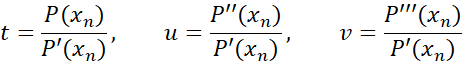
We can now write the householder’s 3rd order as follows:

Characteristic Convergence order Efficiency index for Householder 3rd 4(1/4)=1.41
Householder 3rd order has an efficiency index of 1.41, in line with both Newton and Halley. For each iteration the number of correct digits quadruple.
Equivalent to the Newton method, handling of multiple roots can be done using the Householder 3rd order reduction factor of 3/(m+2) by multiplier the step size with the reverse factor, we should ensure a quartic convergence rate even for multiple roots.
Our modified Householder 3rd order will then be:

Or using the same substitution as before:

From the walkthrough of the Halley iteration, it is clear that we can maintain the same framework and just replace the iteration step. E.g., out with the Halley step and in with the Householder 3rd order.
How the Higher Orders Method Stacks Up Against Each Other
To see how it works with the different methods, let's see the method against a simple Polynomial.
P(x)= (x-2)(x+2)(x-3)(x+3)=x4-13x2+36
The above-mentioned Polynomial is an easy one for most methods. Moreover, as you can see the higher-order method requires fewer numbers of iterations. However, also more work to be done per iteration.
| Method | Newton | Halley | Household 3rd |
| Iterations | Root | Root | Root |
| Start guess | 0.8320502943378436 | 0.8320502943378436 | 0.8320502943378436 |
| 1 | 2.2536991416170737 | 1.6933271400922734 | 2.033435992687734 |
| 2 | 1.9233571772166798 | 1.9899385955094577 | 1.9999990577501767 |
| 3 | 1.9973306906698116 | 1.9999993042509177 | 2 |
| 4 | 1.999996107736492 | 2 | |
| 5 | 1.9999999999916678 | ||
| 6 | 2 |
Here is another example. Consider the polynomial with 6 roots at 1,2,3,4,5,6.
P(x)=x6-21x5+175x4-735x3+1624x2-1764x+720
| Method | Newton | Halley | Householder 3rd |
| Total iterations | 21 | 16 | 14 |
| Ratio | 1 | 0.76 | 0.67 |
| Convergence order | 2 | 3 | 4 |
| Convergence ratio | 1 | 0.67 | 0.5 |
Listed is the total number of iterations for each method. Halley ideally should do the job with only 67% of the required number of iterations for Newton. However, it required 76%. Same for Householder 3rd order that required 67% but ideally should be half the number of Newton iterations. The reason that it does not match up is that convergence order only applies when close to a root. It typically takes a few iterations to get near the root and that is kind of wandering around in the complex plane searching for some tracking to the root. See the below image of the measured convergence order for each method. When tracking happens, each method follows its convergence order.


Other Higher Order Method
There exist other higher-order methods that try to avoid calculating the 2nd and 3rd derivatives in a multi-point schema. For example, the Ostrowski multi-point method has an efficient index of 1.59 and is a 4th-order method. However, you can even find other methods that generate 5, 6, 7, and even 9th order without the use of a derivative. One of the drawbacks is that for many of the multi-point methods, no modified version can deal efficiently with multiple roots.
Despite the multiple root drawbacks, Part Six will deal with the Ostrowski multi-point method and see how we still can incorporate handling of multiple roots efficiently.
In Part Four, we go through Laguerre’s method and in Part Five, we go through one of the simultaneous methods (Weierstrass or Durand-Kerner) that iterate towards all the roots simultaneously.
Recommendation
Since the efficiency index is comparable for these three methods, there are no advantages to using either the Halley or the Householder 3rd order method compared to Newton method. I recommend sticking with the Newton method presented in Parts One and Two.
Conclusion
We have presented a refined Halley method, building upon the framework established in Parts One and Two, to efficiently and stably find roots of polynomials with real coefficients. While Part One focused on polynomials with complex coefficients—where roots could still be real—this second part delves into real coefficients polynomials. Part Three explores adjustments needed for higher-order methods, such as Halley's method, while Part Four will demonstrate the ease of integrating alternative methods like Laguerre's methods into the same framework. A web-based polynomial solver showcasing these various methods is available for further exploration and can be found on http://www.hvks.com/Numerical/websolver.php that demonstrates many of these methods in action.
References
- H. Vestermark. A practical implementation of Polynomial root finders. Practical implementation of Polynomial root finders vs 7.docx (www.hvks.com)
- Madsen. A root-finding algorithm based on Newton Method, Bit 13 (1973) 71-75.
- A. Ostrowski, Solution of equations and systems of equations, Academic Press, 1966.
- Wikipedia Horner’s Method: https://en.wikipedia.org/wiki/Horner%27s_method
- Adams, D A stopping criterion for polynomial root finding. Communication of the ACM Volume 10/Number 10/ October 1967 Page 655-658
- Grant, J. A. & Hitchins, G D. Two algorithms for the solution of polynomial equations to limiting machine precision. The Computer Journal Volume 18 Number 3, pages 258-264
- Wilkinson, J H, Rounding errors in Algebraic Processes, Prentice-Hall Inc, Englewood Cliffs, NJ 1963
- McNamee, J.M., Numerical Methods for Roots of Polynomials, Part I & II, Elsevier, Kidlington, Oxford 2009
- H. Vestermark, “A Modified Newton and higher orders Iteration for multiple roots.”, www.hvks.com/Numerical/papers.html
- M.A. Jenkins & J.F. Traub, ”A three-stage Algorithm for Real Polynomials using Quadratic iteration”, SIAM J Numerical Analysis, Vol. 7, No.4, December 1970.
History
- 10th November, 2023: Initial version