
Summation of Series with Convergence Acceleration
5.00/5 (4 votes)
How to speed up convergence of mathematical series
Introduction
Many applications implements some calculation of a series or sequence that can have a very slow convergence rate or might require more precision than you could get from a brute force implementation. There are several candidates to choose from when implementing these acceleration techniques and I will present the most common ones in this article.
However, there is the the issue that you will not find one universal acceleration technique that will work for all sequences, which is proven mathematically. This proof is based on a property of the sequence called remanence if you are interested in looking it up for yourself. This gives you the hint of either using a mathematical test/prove before releasing it to your costumers or at least your own judgement to test the acceleration technique on the series first. And you should not expect the same magic to work universally.
Background
Assume that we have sequence or series which have the actual (theoretical) sum is \(S\) but we only have the ability to calculate the approximation \(S_n\) :
This analysis can also be used on an infinite product:
So, describing the problem at hand in the most general way, we simply want to minimize the difference \(S - S_n = e\) or if possible to eliminate the error \(e\) . Estimating the form that the error function has and use this information to create a correction is called the kernel, and it is actually the only way we know of making these faster converging or more precise algorithm. If we know how the error grows after each iterative process, we can in fact use this knowledge to predict a better real value then a brute force calculation. And also, since we must guess values that lie beyond what we currently know, we call all these implementations with kernel correcting errors extrapolation methods in mathematics.
Aitken's Summation Formula
Many series that we perform summations on grows geometrical by nature, so at first it seems natural to assume that the error and the correcting kernel can be described by a formula \(b \cdot q^n\). The kernel we want to use in order to try to correct and adjust the complete sum is:
We assume here that \(q < 1\) so that the error actually decrease for each iterative term we sum over in the original series. With the general kernel above we have 3 unknowns \(S, b, q\) in the equation to solve for, which means that we need 3 equations in order to get a unique solution. The result is what is known as Aitken's formula:
The first discoverer of this formula seems to be the Japanese mathematician Takakazu Seki in around 1680. (He is sometimes referred to by mistake as Seki Kowa due to some spelling similarities in Japanese). It has also been discovered independently by others before the name of this way of accelerate the sequence was given to Aitken.
The code is pretty straight forward to implement:
        /// <summary>
        /// Calculates the Aitken summation
        /// </summary>
        /// <param name="S_n">The partial sums of a series</param>
        /// <returns>A extrapolated value for the partial sum</returns>
        /// <exception cref="Exception">If you have less than 3 items,
        /// this will return with an exception</exception>
        public double Aitken(double[] S_n)
        {
            if (S_n.Length > 3)
            {
                double S_2 = S_n[S_n.Length - 1];
                double S_1 = S_n[S_n.Length - 2];
                double S_0 = S_n[S_n.Length - 3];

                return (S_2 * S_0 - S_1 * S_1) / (S_2 -2*S_1 + S_0);
            }
            else
                throw new Exception("Must have at least 3 partial sums
                                     to give the correct value");
        }
Aitkens formula can indeed accelerate all linearly converging series, but in addition, it can also be used to accelerate the much more difficult logarithmic sequences. This algorithm can also be used in multiple stages, meaning that we apply it over and over again on the same summation series.
Shanks Transform and Wynns Epsilon Algorithm
The general acceleration kernel of a geometric series was later formulated into the Shanks transform, were Shanks formulated the correction term with more variables:
This will lead to a 2m +1 unknowns with the general determinant ration found by Shanks in 1947:
Most of the elements in the matrix consists of many finite difference items of consecutive terms, so these elements are usually abbreviated by \( \Delta S_p = S_{p+1} - S_p \). The absolute mark in front and behind the matrix means that you should calculate the determinant of it, and although the determinants can be found by creating a lower (or upper) triangular matrix and simply multiplying the resulting diagonal elements, it does not in general a stable method. The issue here is that the Henkel determinants of matrices on this form uses multiple arithmetical operations that can lead to significant truncation errors when implemented directly on computers. So using a different method is desirable.
There is also a more hidden pattern behind the full Shanks transform of a sequence since it is equivalent to the Pade approximation. One can actually use the Shanks transform to calculate the full Pade approximation, which is also the fastest way of finding a convergence series due to the links to continued fractions. But the same calculation problem remains, we need a better way of calculating this transformation.
Peter Wynn's \(\epsilon\)-algorithm produces the same results by using an iterative process and in fact it is very similar to calculating the continued fraction of a series. We start off by assuming we have a table designated with X,Y were we define 0,0 at the top left corner. In the first column, we fill it with zeros \(\epsilon(0,y) = 0\) and in the second column, we place the partial sum of each iteration \(\epsilon(1,y) = S_n\). We now use the iteration schema below:
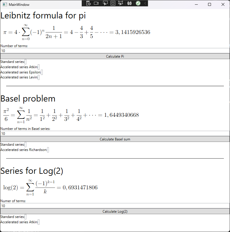
The convergence speedup is used on the slow converging Leibnitz formula for \(\pi\) and can be illustrated with the table in the picture below:

A better, or at least a more common way to illustrate the relation, is to use a lozenge diagram (image taken from https://www.sciencedirect.com/science/article/pii/S0377042700003551#FIG1). The reason is that all values in the lozenge diagram that are used in each of the iterative step is right next to each other in the diagram.

From the calculations, you can see that every even column just contains some intermediary results that is used to calculate the higher degree transformation. These intermediary results are skippable by Wynn cross rule that allows you to only store the odd numbered columns. The issue here is that you need 3 starting columns with the parameters \( \epsilon_{-2}^{(n)} = \infty \),\( \epsilon_{-1}^{(n)} = 0 \) and finally \( \epsilon_{0}^{(n)} = S_n \) to implement the iterative process below:
There is no real advantage to implement this algorithm on a computer, except that it eliminates columns that have the intermediate calculation results, but it has the drawback or disadvantage of needing one more starting condition. The more interesting thing that could be mentioned is that Wynn also found an implementation that can calculate the accelerated sums with just one vector and two intermediary variables. But on the modern computer this is not an issue and I will skip this derivation. You might have guessed it already, but Peter Wynn's \(\epsilon\)-algorithm could also be used to calculate the Hankel determinant, the Pade approximation and surprisingly also be used to solve the differential wave type equation called Korteweg–De Vries (KdV) equation.
Now we switch to the actual implementation of the code, and first off, we need the test series that the acceleration algorithm shall accelerate. We have already previously illustrated the algorithms usefulness with the slowly converging series that Leibnitz found for pi given by the series:
The sum following each new term of the truncated series is saved in a list and returned.
        public static double[] PartialSumPi_Leibnitz(int n = 6)
        {
            double sum = 0;
            double sign = 1;
            double[] result = new double[n];
            int ind = 0;
            for (int i = 1; i < n*2; i= i+2)
            {
                sum = sum + sign * 4 / i;
                sign *= -1;
                result[ind] = sum;
                ind += 1;
            }
            return result;
        }
The actual code for Wynn's algorithm is given below:
        /// <summary>
        /// Peter Wynns epsilon algorithm for calculating accelerated convergence
        /// </summary>
        /// <param name="S_n">The partial sums</param>
        /// <returns>The best accelerated sum it finds</returns>
        public static double EpsilonAlgorithm(double[] S_n, bool Logaritmic = false)
        {

            int m = S_n.Length;

            double[,] r = new double[m + 1, m + 1];

            // Fill in the partial sums in the 1 column
            for (int i = 0; i < m; i++)
                r[i, 1] = S_n[i];

            // Epsilon algorithm
            for (int column = 2; column <= m; column++)
            {
                for (int row = 0; row < m - column + 1; row++)
                {
                    //Check for divisions of zero (other checks should be done here)
                    double divisor = (r[row + 1, column - 1] - r[row, column - 1]);

                    // Epsilon
                    double numerator = 1;

                    if (Logaritmic)
                        numerator = column + 1;

                    if (divisor != 0)
                        r[row, column] = r[row + 1, column - 2] + numerator / divisor;
                    else
                        r[row, column] = 0;
                }
            }

            // Clean up, only interested in the odd number columns
            int items = (int)System.Math.Floor((double)((m + 1) / 2));
            double[,] e = new double[m, items];

            for (int row = 0; row < m; row++)
            {
                int index = 0;
                for (int column = 1; column < m + 1; column = column + 2)
                {
                    if (row + index == m)
                        break;

                    //e[row + index, index] = r[row, column];
                    e[row, index] = r[row, column];
                    index += 1;
                }
            }
            return e[0, e.GetLength(1) - 1];
        }
Other algorithms based on the \(\epsilon\)-algorithm have been proposed like the \(\rho\)-algorithm also by Wynn:
Here the \( x_n \) is the interpolation points used in the sequence. In the usual case of integer sums the simplification \( x_n = n + 1\) is used.
These algorithms generally works better for accelerating series that have logarithmically increasing errors.
Richardson Extrapolation and Euler's Alternating Series Transformation
Two similar methods for faster convergence that are often not grouped together, even though Richardson extrapolation is calculated with Taylor expansion and the Euler transform by finite difference approximation by a devilishly clever trick from its inventor Euler. We start off with the well known Taylor expansion of the unknown \( f(x) \) were the function is adjusted by a small amount \( h \). And by the way. Taylor expansion is every mathematicians favorited method in applied mathematics. Not a day goes by without using it. Well, almost none anyway, so here it is incase you had forgotten it:
In the Richardson extrapolation we utilize the structure of the Taylor series with different multiple values of \( h \) as \( 2h, 3h, \cdots \). This information is used by a system of equations that allows us to eliminate higher and higher order derivatives in the Taylor expansion. In the generalized Richardson extrapolation, we take the idea of the Taylor expansion and use the integer sum the value \( \frac{1}{n} \) is used instead of \( h \) and reformulate the sum with the error estimate:
The resulting closed form solution equations, that will give us a unique solution, are set up in the equations below. (Derivation and result is taken from "Advanced mathematical methods for scientists and engineers" by Bender ang Orszag)
Solving for \(S\) gives the solution to the m equations:
The code for the Richardson extrapolation have the weakness in the dependence of the factorial, effectively limiting higher order implementations on the computer:
        /// <summary>
        /// Generalized Richardson extrapolation
        /// </summary>
        /// <param name="S_n">The partial sums</param>
        /// <returns>Best approximation of S</returns>
        public static double RichardsonExtrapolation(double[] S_n)
        {
            double S = 0d;

            double m = S_n.Length;
            for (int j = 1; j <= (int)m; j++)
            {
                S += System.Math.Pow(-1, m + (double)j) *
                    S_n[j - 1] *
                    System.Math.Pow((double)j, m - 1)
                    / (Factorial(j - 1) * Factorial(m - j));
            }

            return S;
        }
The next item to showcase is the Euler series transformation that are usually applied to an alternating series on the form:
The Euler transformation of the series above is given below:
Here the general difference formula is defined as:
What is actually happening here, and Euler's brilliant insight, is that the alternating series could be written out as:
By the way, you can always count on Euler beings astoundingly simple and brilliant. It there is a simple solution a problem he will find it in most cases. Doing the transformation on the alternating series multiple times effectively implies that we use higher and higher order of finite difference and getting a better and better approximation each time.
Actually the difference between Taylors formula and the finite difference equivalent can be illustrated by the exponential number \( e \) from calculus and the difference equivalent 2:
The underline in the power \(X^{\underline{2}}\) is called falling powers:
The formula is quite general, you can even plug in rational numbers like \( 2^{\frac{1}{2}} = \sqrt{2}\) and the formula still works. This was Newtons big insight into the binomial coefficients allowing him to calculate the square root of numbers.
Now for the code that performs the Euler transformation is given below:
        /// <summary>
        /// Euler transform that transforms the alternating series
        /// a_0 into a faster convergence with no negative coefficients
        /// </summary>
        /// <param name="a_0">The alternating power series</param>
        /// <returns></returns>
        public static double[] EulerTransformation(double[] a_0)
        {
            // Each series item
            List<double> a_k = new List<double>();

            // finite difference of each item
            double delta_a_0 = 0;

            for (int k = 0; k < a_0.Length; k++)
            {
                delta_a_0 = 0;
                for (int m = 0; m <= k; m++)
                {
                    double choose_k_over_m = (double)GetBinCoeff(k, m);
                    delta_a_0 += System.Math.Pow(-1d, (double)m) *
                                 choose_k_over_m * System.Math.Abs(a_0[(int)(m)]);
                }

                a_k.Add(System.Math.Pow(1d / 2d, (double)(k + 1)) * delta_a_0);
            }
            return a_k.ToArray();
        }
It is also possible to use Euler's series transformation on series that are not alternating, with the help of some conversion algorithm:
where the altered series is the following transformation:
Levin's Transformation
Levin's transformation is based on the assumption that one chooses b larger than zero and the remainder estimate \( \omega_m \) is suitably chosen for the series that one wants to accelerate:
The resulting formula is given below:
The code implementation of the Levin algorithm:
        /// <summary>
        /// Levins algorithm L_{k}^{n}(S_n) but k + n has to be less than
        /// the length of S_n minus one
        /// </summary>
        /// <param name="S_n">The partial truncated sums</param>
        /// <param name="k">The 'order' of Levins algorithm</param>
        /// <param name="n">The n'th point approximation</param>
        /// <returns>The accelerated value</returns>
        public static double LevinsAlgorithm(double[] S_n, double k = 4, double n = 5)
        {
            double numerator = 0;
            double denominator = 0;

            if (k + n > S_n.Length - 1)
                throw new ArgumentException("Not enough elements to
                      sum over with the n'th element with order k");

            for (int j = 0; j < n ; j++)
            {
                double rest = System.Math.Pow(-1d, j) *
                              GetBinCoeff((double)k, (double)j);

                double C_jkn_U = System.Math.Pow((double)(n + j + 1), k - 1);
                double C_jkn_L = System.Math.Pow((double)(n + k + 1), k - 1);

                double C_njk = C_jkn_U / C_jkn_L;

                double S_nj = S_n[(int)n + (int)j];

                // t transform that calculates a_n
                double g_n = S_n[(int)n + j] - S_n[(int)n + j - 1];
                // u transform that calculates (n+k) * a_n
                // g_n = (n + k)* (S_n[(int)n + j] - S_n[(int)n + j - 1]);

                numerator += rest * C_njk * S_nj / g_n;
                denominator += rest * C_njk / g_n;
            }

            return numerator / denominator;
        }
References
Books
- Advanced Mathematical Methods Scientists Engineers
- Asymptotic Analysis Perturbation - William Paulsen
- Numerical Analysis - Historical Developments in the 20th Century
Other Online Sources
- Eulers acceleration transform
- Accelerating Convergence of Series
- NIST Digital Library of Mathematical Functions
- Euler transformation from Encyclopedia of Math - Springer
History
- 9th February, 2023: Initial version