
Python Fourier Transform Helper Library
5.00/5 (11 votes)
A Python Library to help make properly scaled Fourier Transforms including utility functions
Introduction
There is a real need in Python 3 for a ready-to-use Fourier Transform Library that users can take right out of the box and perform Fourier Transforms (FT), and get a classical, properly scaled spectrum versus frequency plot.
The vast majority of code that you will find in Commercial packages, Open Source libraries, Textbooks, and on the Web is simply unsuited for this task and takes hours of further tweaking to get a classic and properly scaled spectrum plot. You know: Proper “Amplitude” and no more “Negative frequencies”, etc.
What “Fourier Transform Helper Lib” Does
FourierTransformHelperLib.py (FTHL) has several main parts, but its basic goal is to allow a real Fourier Transform to be performed on a real or complex time series input array, resulting in a usable classic spectrum output without any further tweaking required by the user [1].
Step by step examples are given for many use cases showing how to:
- generate test signals (which can be replaced by your real signals later).
- properly apply a Window to the input data, using any of the 32 included windows.
- perform the Fourier Transform.
- properly scale the Fourier Transform to correct for the applied Window in Step 2.
- convert the Fourier Transform to Magnitude or dBV format.
- plot a nice frequency amplitude display of the real frequencies (i.e., a Classical Spectrum Plot)
What “Fourier Transform Helper Lib” Does Not Do
With all this windowing, scaling, and slicing of the raw Fourier Transform data into a usable positive frequency only display, it is not possible to go backward and perform a proper Inverse Fourier Transform on the FFT output. This is because of the way the Fourier Transforms work. The transforms basic math requires that the total energy in a forward and inverse transform be maintained [2]. After all the windowing, scaling, etc. This would have to be backed out somehow to get back to the original signal and this is not the purpose of this library at all. As shown above, the purpose of this library is to make a usable and correctly scaled Forward Transform with the minimum user required steps.
Under the Hood
Basic Fourier Transforms (FT) come in two basic types: The most general form can produce a spectrum output from any length of input data. This type of transform is called the Discrete Fourier Transform or DFT. The DFT code is simple and brute force.
The pros are: The input data can be any length.
The cons are: Since it is a general method, it is computationally intensive and large input data sets can take a very long time to calculate.
A more specific type of FT is called the Fast Fourier Transform or FFT.
The pros are: It is much, much faster to compute than the DFT.
The cons are: The input data length is constrained to be powers of two. The code is more complex to understand.
As an example: A 65536 point Python FFT takes about 1.3 Milliseconds on my 4 GHz, i7 Core Computer. A DFT of length 65535 takes 3.9 Milliseconds. That’s around 3 times slower for a one-point change in input signal length!
FTHL implements both kinds of Fourier Transform on real and complex input data by basing the transform on the SciPy.FFT package transform. SciPy.FFT will select the appropriate transform type depending on the input data length, so you don’t have to worry about it. Just keep in mind: If speed is the main concern:
- Make your data set as small as possible.
- Make your data set length a power of two (i.e., 1024, 2048, 4096, etc.).
Note: For the remainder of this article, the generalized Fourier Transform will be referred to as an 'FT' when the discussion can apply to either an 'FFT' or 'DFT' as they both produce the same result for equivalent input data.
Real and Imaginary Spectrum Parts
All FT implementations naturally produce an output data array that is the same length as the input array. The output however consists not only of complex numbers but Real and Imaginary parts of the Spectrum itself – sometimes called negative frequencies depending on how one wants to think about it. The Negative Frequencies part of the spectrum is normally just the mirror image of the Real part and does not contain any additional information about the spectrum.
FTHL returns only the real part of the spectrum output data array (roughly one-half the length of the input data array). All the other libraries that you will find give you the entire Real and Negative frequency parts as a return value, including SciPy’s FFT module. This is a source of confusion for many people and it is not useful for generating the usual real spectrum data representation.
Note: If you need the Negative and Real parts of the complex spectrum for some mathematical reason, that's fine, you know why you need it. FTHL is geared towards generating scaled classical spectrum plots, not general FT mathematics.
Fourier Transform Scaling
Most of the FT implementations you will find are not scaled properly for classical spectrum displays. That is, the amplitude of a transformed signal varies with the number of transformed points: N. This is disconcerting to most users. Most users expect a properly scaled output independent of the number of points used in the FT.
For instance, if a user inputs a 10 Hz signal of 1 Vrms amplitude, then they expect to see a 1 Vrms peak at 10 Hz in the spectrum plot. FTLH is the only Python 3 library to date that properly scales the FT outputs so that they are accurate, no matter how you change the number of points in the transform, or what window you use on the input data.
Note: All FT implementations also have scaling differences at DC (Bin 0) and one-half the Sampling Frequency. These points have no imaginary part, only a real part. Hence, the required scaling is different at these points also. FTHL applies the proper scale to the DC Bin also.
Scaling with Added Data Windowing
You may know that all FTs assume that the chunk of time-limited data that you input extends for an infinite time both before the chunk and afterward. If you transform a pure sine wave with an even number of cycles, the spectrum display will be a perfect peak centered in one bin of the output spectrum.
In real life, it is usually not possible to generate exactly even input sequences. Any fractional cycles and the output will be smeared across the entire resulting spectrum. The amplitude of fractional cycles, or peaks in-between FT Bins will also appear to be lower than they actually are.
This is where using a window comes into play. A window is applied to the input data and it tapers the beginning and end of the time series to zero or near zero. The use of a window thus tricks the FT into not noticing the discontinuities in the input data.
Windows are normally picked based on four criteria:
- How low in amplitude they push the undesired sidelobes.
- How much do they reduce the amplitude uncertainty.
- How many adjacent FT Bins do they "smear" the data into.
- Historical reasons, i.e., "Everybody uses Window: "XYZ", in this situation.", etc.
Picking the optimum window involves many tradeoffs.
FTHL’s windowing is based on an excellent article written by the staff at the Max Planck Institute [3] and includes all the usual types of windows like Welch, Hamming, and Hann (or Hanning as it is commonly called) and 29 other very useful but perhaps less well-known windows. Also included are 17 very unique Flat Top windows that give very low amplitude error even if the input frequency is in between the FT output Bins.
Since Windowing the input data changes it physically, it can also change the resulting FT Spectrum output amplitudes. FTHL includes two functions that allow the window gain (or loss) to be accounted for so that the properly scaled FT output can be found and displayed. One of the scale factors relates to the peak of discrete signals. The other type of scale factor must be used when noise is being measured.
After a set of window coefficients is generated, they are input to the appropriate Scale Factor functions(s) and a scalar scale factor number is calculated. This scale factor is applied by multiplication to the resulting FT Magnitude spectrum data to correct the amplitude.
More information on the need and selection of windows may be found in reference [3].
Zero Padding and Scaling
Zero padding is a very useful trick that is used with FTs. One use is to round the length of input data up to the next power of two so that a faster FFT can be used for the transform method. For instance, if you had 1000 points of input data, you can “zero pad” an additional 24 points of zero’s data onto the original data so that a 1024 point FFT can be performed instead of a slower 1000 point DFT.
Another use for zero padding is to make the display look more like an expected spectrum display. Zero padding broadens any peak(s) by interpolating points on the display and this makes a plot look better on a display screen or a plot. Zero padding also interpolates the space between calculated points reducing amplitude error when signals are not directly at the bin centers of the FT.
Finally, zero-padding allows a very fine look at the sidelobes and sideband suppression added by the window.
Zero padding also influences the resulting spectrum output amplitudes even when the signals are at the bin centers. The FT routine presented here takes into consideration the desired zero-padding number so that the proper re-scaling factors can automatically be taken into account. Since the FT routines know about the desired zero padding for scaling reasons, they add the requested amount of zeros to the input data so the user does not have to.
Reference [4] has more information on Zero Padding and even more uses for it.
Test Data Generation
Real data to analyze isn't always available during program development and debugging. FTHL helps by including calibrated Sine Wave generators and calibrated Gaussian Random Noise generators for making lifelike test signals that can also include noise.
General Spectrum Output Manipulation Methods
As mentioned, the raw output of any FT is an array of complex numbers. In addition to the Python 3’s Complex number type operators in the cmath library, FTHL includes several easy-to-use conversion routines for converting the Complex result into a scalar array of either Linear, Linear Squared, or Log Magnitude dBV formats [5].
Using the Code
Enough talk about the general aspects of Fourier Transforms and the FTHL. The examples below will show how easy it is to apply in practice.
Example 1 – Basic Setup for Making a Fourier Transform on an Input Signal
import FourierTransformHelperLib as ft
import matplotlib.pyplot as plt

"""
FourierTransformHelperLib - Article Example 1
Generate a test signal and produce a properly scaled spectrum magnitude output
"""

# Generate a 5001 Hz Test Signal Tone with a 1.0 VRMS Amplitude
time, sig = ft.tone_sampling_points
      (amplitude=1.0, frequency=5001, sampling_frequency=20000, points=200, phase=0)

# Perform Fourier Transform and convert amplitude to magnitude
ft_sig = ft.ft_cpx(sig)
y = ft.complex_to_mag(ft_sig)

# Get X Scale of frequencies for plotting
x = ft.frequency_bins(sampling_rate=10000, signal_length=len(sig))

# Plot Spectrum
plt.figure(2)
plt.semilogy(x, y)

plt.title('Scaled Spectrum')
plt.xlabel('Frequency [Hz]')
plt.ylabel('Amplitude [Vrms]')
plt.show()
In the example above, a test signal is generated, and the FT is executed. Scaling is done on the result and the spectrum magnitude result is available for plotting in the arrays: x, and y. Notice how few lines of code it takes to generate the test signal, transform it, and convert the complex FT output into a usable magnitude format for plotting.

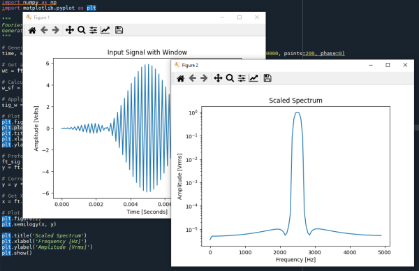
Example 2 – Applying a window to the input data first, tricks the FT into thinking that the Waveform Discontinuities are not there
import FourierTransformHelperLib as ft
import matplotlib.pyplot as plt

"""
FourierTransformHelperLib - Article Example 2
Generate a signal, window it, and produce a properly scaled spectrum magnitude output
"""

# Generate a 5001 Hz Test Signal Tone with a 1.0 VRMS Amplitude
time, sig = ft.tone_sampling_points(amplitude=1.0, frequency=5001,
                                    sampling_frequency=20000, points=200, phase=0)

# Get a window for the input data (Window)
wc = ft.window(window_type='fthp', points=len(sig))

# Calculate the sale factor of this generated window (Window)
w_sf = ft.window_scale_signal(window_coefficients=wc)

# Apply window to data (Window)
sig_w = sig * wc

# Plot input signal w/window
plt.figure(1)
plt.plot(time, sig_w)
plt.title('Input Signal with Window')
plt.xlabel('Time [Seconds]')
plt.ylabel('Amplitude [Volts]')

# Perform Fourier Transform and convert amplitude to magnitude
ft_sig = ft.ft_cpx(sig_w)
y = ft.complex_to_mag(ft_sig)

# Correct signal amplitude for window (Window)
y = y * w_sf

# Get X Scale for plotting
x = ft.frequency_bins(sampling_rate=10000, signal_length=len(sig))

# Plot Spectrum
plt.figure(2)
plt.semilogy(x, y)

plt.title('Scaled Spectrum')
plt.xlabel('Frequency [Hz]')
plt.ylabel('Amplitude [Vrms]')
plt.show()
To apply a window to the input data only takes 4 more lines of code as shown above (these lines are commented with (Window) in the code above. Compare the code for example 2 above to the code given for example 1.


Example 3 – Transform With Window and Zero Padding
import FourierTransformHelperLib as ft
import matplotlib.pyplot as plt

"""
FourierTransformHelperLib - Article Example 3
Generate a signal, window it, add zero padding to the FT,
and produce a properly scaled spectrum magnitude output
"""

# Generate a 5001 Hz Test Signal Tone with a 1.0 VRMS Amplitude
time, sig = ft.tone_sampling_points(amplitude=1.0, frequency=5001,
                                    sampling_frequency=20000, points=200, phase=0)

# Get a window for the input data
wc = ft.window(window_type='fthp', points=len(sig))

# Calculate the sale factor of this generated window
w_sf = ft.window_scale_signal(window_coefficients=wc)

# Apply window to data
sig_w = sig * wc

# Plot input signal w/window
plt.figure(1)
plt.plot(time, sig_w)
plt.title('Input Signal with Window')
plt.xlabel('Time [Seconds]')
plt.ylabel('Amplitude [Volts]')

# Perform Fourier Transform and convert amplitude to magnitude
# Add the desired zero padding here (Padding)
ft_sig = ft.ft_cpx(sig_w, zero_padding=2000)
y = ft.complex_to_mag(ft_sig)

# Correct signal amplitude for window
y = y * w_sf

# Get X Scale (Remember that you added zero padding, so the length will be longer)
# (Padding)
x = ft.frequency_bins(sampling_rate=10000, signal_length=len(sig),
                      zero_padding_length=2000)

# Plot Spectrum
plt.figure(2)
plt.semilogy(x, y)

plt.title('Scaled Spectrum')
plt.xlabel('Frequency [Hz]')
plt.ylabel('Amplitude [Vrms]')
plt.show()
In the example 3 code above, to add zero padding to the code of example two only takes the modification of two lines, marked in the comments of the code above as: (Padding)

Review of Basic Usage Steps for Using FTHL
FTHL was designed to be consistent in its use. Additionally, Signals and Noise signals can be analyzed following the same basic steps, as outlined below.
Basic Usage Steps - Analysis of Signal Magnitude
- Calculate window coefficients and window scale factor for signals.
- Get or generate input data.
- Apply window to input data.
- Execute the FT on windowed input data.
- Convert to magnitude format.
- Apply window scale factor to data.
Result: Properly scaled Spectrum for Signals
Basic Usage Steps - Analysis of Noise Signal
- Calculate window coefficients and window scale factor for signals.
- Get or generate input data.
- Apply window to input data.
- Execute the FT on windowed input data.
- Convert to magnitude squared format.
- If required: Average Magnitude Squared data bin by bin, then repeat steps 2-6 for all averages.
- Convert to magnitude format.
- Apply window scale factor to data.
Result: Properly scaled Spectrum for Noise Signals.
Note: The reason why signals and noise must be treated differently are outlined in references [3] and [4].
Description of Test Application & Examples
The code download includes the FTHL Python file, and eight example test scripts, or cookbooks, that show how to do various common transform use cases. These cookbook examples should be very helpful in getting FTHL running for your particular needs.
Example code cookbooks provided in the download above:
Example 1 – A basic DFT Example that generates data and produces a spectrum output
Example 2 – Same as #1 above, but applying a window to the test data
Example 3 – Same as #2 above, but adds zero padding
Example 4 – Same as #2 above, but uses final scaling of dBV [4] for the display
Example 5 – Explains the proper way to generate and average noise
Example 6 – Signal with noise floor added to simulate a real signal
Example 7 – Demonstrates how to extract phase information from the FT output
Example 8 – Demonstrates how to perform a complete FT on Complex IQ input data
Complete Library Documentation
A complete Library Description of each section and function of FTHL is presented below. The library also implements Python Doc String Comments that enable “Real-Time” help in most Python IDEs.
Basic Fourier Transform Core Function
Converts an input data array of real or complex numbers into a properly scaled, and sliced complex output. The parameter zero_padding is optional and if included will append that many zeros to the input data length. Note: The FT has to know about the number of zeros added to do the proper scaling on the result.
def ft_cpx(signal, zero_padding=0):
    """
    Performs Fourier Transform on the input signal.
    Input may be real or complex.
    Input may be any length (not just powers of two).
    Uses SciPy.FFT as the base FFT implementation.

    Args:
        signal (float or Complex array): Input Signal to transform.
        zero_padding (int, optional): Additional zeros to pad the signal with
        Defaults to 0.

    Returns:
        complex: Resulting Fourier Transform as complex numbers.
        sliced to real frequencies only.
    """
Frequency Span Calculation
This function takes the signal length (plus any zero padding that you added to the FT) and calculates an array of the frequencies for each of the points returned by the FT function above. This is useful for making the x-axis of a plot.
def frequency_bins(sampling_rate, signal_length, zero_padding_length=0):
    """
    Calculates the frequency of each Fourier Transform bin.
    Useful for plotting x axis of a Fourier Transform.

    Args:
        sampling_rate (float): Sampling Frequency in Hz
        signal_length (int): Length of input signal
        zero_padding_length (int, optional): Zero padding length. Defaults to 0.

    Returns:
        float array: Array of frequencies for each of the Fourier Transform Bins.
    """
Fourier Transform Format Conversion
This group of functions converts the Complex or Real data array output of the complex FT output to more convenient end-user formats. The example cookbooks included in the download show most of these format conversions and how they are used. Several output formats are available:
def complex_to_mag(cpx_arry):
    """Convert Complex Array to Magnitude Format Array.

    Args:
        cpx_arry (complex array): Complex Input Array.

    Returns:
        float array: Magnitude Format Output.
    """
def complex_to_mag2(cpx_arry):
    """Convert Complex Array to Magnitude Squared Format Array.

    Args:
        cpx_arry (complex array): Complex Input Array.

    Returns:
        float array: Magnitude Squared Format Output.
    """
def complex_to_dBV(cpx_arry):
    """Convert Complex Array to dBV Format Array.

    Args:
        cpx_arry (complex array): Complex Input Array.

    Returns:
        float array: dBV Format Output.
    """
def mag_to_mag2(mag_arry):
    """Convert Float Array to Magnitude Squared Format Array.

    Args:
        mag_arry (float array): Float Input Array.

    Returns:
        float array: Magnitude Squared Format Output.
    """
def mag_to_dBV(mag_arry):
    """Convert Float Array to dBV Format Array.

    Args:
        mag_arry (float array): Magnitude Input Array.

    Returns:
        float array: dBV Format Output.
    """
def mag2_to_mag(mag2_arry):
    """Convert Magnitude Squared Float Array to Magnitude Format Array.

    Args:
        mag2_arry (float array): Magnitude Squared Input Array.

    Returns:
        float array: Magnitude Format Output.
    """
def mag2_to_dBV(mag2_arry):
    """Convert Magnitude Squared Float Array to dBV Format Array.

    Args:
        mag2_arry (float array): Magnitude Squared Input Array.

    Returns:
        float array: dBV Format Output.
    """
def complex_to_phase_degrees(cpx_arry):
    """Convert Complex Number Input To Equivalent Phase Array In Degrees

    Args:
        cpx_arry (complex array): Input Array Of Complex Numbers.

    Returns:
        float array: Resulting Phase Angle In Degrees of Each Input Point
    """
def complex_to_phase_radians(cpx_arry):
    """Convert Complex Number Input To Equivalent Phase Array In Radians

    Args:
        cpx_arry (complex array): Input Array Of Complex Numbers.

    Returns:
        float array: Resulting Phase Angle In Radians of Each Input Point
    """
Note: The calculated phase always has discontinuities at +/-PI intervals. To prevent this, the numpy.unwrap() function can be used to attempt to unwrap the input phase arrays to remove jump-type discontinuities. This works well for clean signals, but as the signal-to-noise ratio declines, it is harder to determine the true discontinuities from noise. The function numpy.unwrap() is a good starting point, but with real-world signals and low signal-to-noise ratios, the best performance is when sufficient signal averaging is used (see example 5 in the download above).
Window Coefficient Generation
The windows are specified with a string value of the desired window name. This is passed into the function Coefficients along with the number of points desired. The result is an array of doubles that can be applied by multiplying with the input data and also used by one of the scaling factor routines to determine the window gain or loss. The window names and parameters are specified in Appendix A below and also provided in a text file list in the download package above.
Note: Do not add any zero padding to the window length generated here.
def window(window_type, points):
    """
    Generates the window coefficients for the specified window type.

    Parameters
    ----------
    window_type : string
        One of the following types of window may be specified,
    points : int
        Number of points total to generate.

    Returns
    -------
    numpy array of the generated window coefficients.
    Returns empty list if error.

    """
Window Analysis and Scaling
Given any set of window coefficients, these routines will determine the gain or loss of the supplied window data array. The window coefficients can be from any window, they are not limited to only the windows supplied by FTHL.
The window_scale_noise function also takes into account the bin width in Hz to correct for multiple or fractional hertz bin widths. See Example 5 in the download package for more information on how to use this.
The function noise_bandwidth function calculates the normalized, equivalent noise bandwidth of the supplied window coefficients in bins [3].
def window_scale_signal(window_coefficients):
    """
    Calculate Signal scale factor from window coefficient array.
    Designed to be applied to the "Magnitude" result.

    Args:
        window_coefficients (float array): window coefficients array

    Returns:
        float: Window scale correction factor for 'signal'
    """
def window_scale_noise(window_coefficients, sampling_frequency):
    """
    Calculate Noise scale factor from window coefficient array.
    Takes into account the bin width in Hz for the final result also.
    Designed to be applied to the "Magnitude" result.

    Args:
        window_coefficients (float array): window coefficients array
        sampling_frequency (_type_): sampling frequency in Hz

    Returns:
        float: Window scale correction factor for 'signal'
    """
def noise_bandwidth(window_coefficients):
    """
    Calculate Normalized, Equivalent Noise BandWidth from window coefficient array.

    Args:
        window_coefficients (float array): window coefficients array

    Returns:
        float: Equivalent Normalized Noise Bandwidth
    """
Signal Generation
These routines can be used to generate test signals for simulation purposes.
def tone_cycles(amplitude, cycles, points, phase):
    """
    Generates a sine wave tone, of a specified number of whole or partial cycles.

    Parameters
    ----------
    amplitude : float
        The desired amplitude in RMS volts.
    cycles : float
        The number of whole or partial sinewave cycles to generate.
    points : int
        Number of points total to generate.
    phase : float
        Phase angle in degrees to generate. The default is 0.0.

    Returns
    -------
    numpy array of the generated tone values.

    """
def tone_sampling_points(amplitude, frequency, sampling_frequency, points, phase):
    """
    Generates a sine wave tone, like it would be if sampled at a specified
    sampling frequency.

    Parameters
    ----------
    amplitude : float
        The desired amplitude in RMS volts.
    frequency : float
        Frequency in Hz of the generated tone.
    sampling_frequency : float
        Sampling frequency in Hz.
    points : int
        Number of points to generate.
    phase : float
        Phase angle in degrees to generate.

    Returns
    -------
    numpy tuple array of the time scale (x) and generated tone values (y).

    """
def tone_sampling_duration(amplitude, frequency, sampling_frequency, duration, phase):
    """
    Generates a sine wave tone, like it would be if sampled at a specified
    duration.

    Parameters
    ----------
    amplitude : float
        The desired amplitude in RMS volts.
    frequency : float
        Frequency in Hz of the generated tone.
    sampling_frequency : float
        Sampling frequency in Hz.
    duration : float
        Number of seconds to generate.
    phase : float
        Phase angle in degrees to generate.

    Returns
    -------
    numpy tuple array of the time scale (x) and generated tone values (y).

    """
The noise routines generate calibrated noise signals depending on the application requirements. Either a Power Spectral Density may be specified (PSD) or a Volts RMS value for noise may be used.
The units for Power Spectrial Density (PSD) are Vrms / rt-Hz (Read as: Volts RMS Per Root-Hertz).
def noise_psd(amplitude_psd, sampling_frequency, points):
    """
    Generates a random noise stream of a given power spectral density
    in Vrms/rt-Hz. The noise is normally distributed, with a mean of 0.0 Volts.

    Parameters
    ----------
    density : float
        The desired noise density of the generated signal Vrms/rt-Hz.
    sampling_frequency : float
        Sampling frequency in Hz.
    number : int
        Number of points total to generate.

    Returns
    -------
    numpy array of the generated noise.

    """
def noise_rms(amplitude_rms, points):
    """
    Generates random noise stream of a given RMS voltage.
    The noise is normally distributed, with a mean of 0.0 Volts.

    Parameters
    ----------
    amplitude : float
        The desired amplitude in Volts RMS units..
    number : int
        Number of points total to generate.

    Returns
    -------
    numpy array of the generated noise.

    """
Using the “Fourier Transform Helper Library” in your Projects
Download FTHL_source_and_examples.zip from the link above. This zip file contains the FourierTransformHelperLib.py source file, and all the example scripts.
The simplest usage is to place the file FourierTransformHelperLib.py into your project directory, as that way Python is sure to find it.
Add the FourierTransformHelperLib.py source file as an “import” to your project as shown below:
import FourierTransformHelperLib as ft
System Requirements
The FourierTransformHelperLib.py was developed and tested with python 3.9+ and the modules: numpy 1.22.2, and scipy 1.8.0.
References
[1] Steve Hageman, “DSPLib - FFT / DFT Fourier Transform Library for .NET 4”,
https://www.codeproject.com/Articles/1107480/DSPLib-FFT-DFT-Fourier-Transform-Library-for-NET-6
[2] Parseval's theorem,
https://en.wikipedia.org/wiki/Parseval%27s_theorem
[3] G. Heinzel, A. Rudiger, and R. Schilling, “Spectrum and spectral density estimation by the Discrete Fourier transform (DFT), including a comprehensive list of window functions and some new flat-top windows.”, Max-Planck-Institut fur Gravitationsphysik, February 15, 2002
[4] Steve Hageman, "The practicing instrumentation engineer's guide to the Fourier Transforms", Published on EDN.com, June 2012.
Part 1: Understand DFT and FFT implementations
Part 2: Spectral leakage and windowing
Part 3: Other window types, averaging DFTs & more
Measuring small signals accurately: A practical guide
[5] dBV refers to a 20 * logarithmic scale of dB (Decibels) referred to 1 Volt RMS. Example,
10 V RMS = 20 dBV
1 V RMS = 0 dBV
0.1 V RMS = - 20 dBV
See aso: https://en.wikipedia.org/wiki/Decibel
Appendix A – Included Window Types
Below are the tabulated performance parameters of the windows implemented in FTHL.
For more information on these windows, see Reference [3].
Name Peak Sideband Level (dB) Flatness (dB) 3dB BW (bins) NENBW (bins)
| Name | Peak Sideband Level (dB) | Flatness (dB) | 3dB BW (bins) | NENBW (bins) |
| Rectangular or None | 13.3 | 3.9224 | 0.8845 | 1 |
| Welch | 21.3 | 2.2248 | 1.1535 | 1.2 |
| Bartlett | 26.5 | 1.8242 | 1.2736 | 1.3333 |
| Hanning or Hann | 31.5 | 1.4236 | 1.4382 | 1.5 |
| Hamming | 42.7 | 1.7514 | 1.3008 | 1.3628 |
| Nuttall3 | 46.7 | 0.863 | 1.8496 | 1.9444 |
| Nuttall4 | 60.9 | 0.6184 | 2.1884 | 2.31 |
| Nuttall3A | 64.2 | 1.0453 | 1.6828 | 1.7721 |
| Nuttall3B | 71.5 | 1.1352 | 1.6162 | 1.7037 |
| Nuttall4A | 82.6 | 0.7321 | 2.0123 | 2.1253 |
| BH92 | 92 | 0.8256 | 1.8962 | 2.0044 |
| Nuttall4B | 93.3 | 0.8118 | 1.9122 | 2.0212 |
Table 1 - Normal Windows implemented in FTHL.
| Name | Peak Sideband Level (dB) | Flatness (dB) | 3dB BW (bins) | NENBW (bins) |
| SFT3F | 31.7 | 0.0082 | 3.1502 | 3.1681 |
| SFT3M | 44.2 | 0.0115 | 2.9183 | 2.9452 |
| FTNI | 44.4 | 0.0169 | 2.9355 | 2.9656 |
| SFT4F | 44.7 | 0.0041 | 3.7618 | 3.797 |
| SFT5F | 57.3 | 0.0025 | 4.291 | 4.3412 |
| SFT4M | 66.5 | 0.0067 | 3.3451 | 3.3868 |
| FTHP | 70.4 | 0.0096 | 3.3846 | 3.4279 |
| HFT70 | 70.4 | 0.0065 | 3.372 | 3.4129 |
| FTSRS | 76.6 | 0.0156 | 3.7274 | 3.7702 |
| SFT5M | 89.9 | 0.0039 | 3.834 | 3.8852 |
| HFT90D | 90.2 | 0.0039 | 3.832 | 3.8832 |
| HFT95 | 95 | 0.0044 | 3.759 | 3.8112 |
| HFT116D | 116.8 | 0.0028 | 4.1579 | 4.2186 |
| HFT144D | 144.1 | 0.0021 | 4.4697 | 4.5386 |
| HFT169D | 169.5 | 0.0017 | 4.7588 | 4.8347 |
| HFT196D | 196.2 | 0.0013 | 5.0308 | 5.1134 |
| HFT223D | 223 | 0.0011 | 5.3 | 5.3888 |
| HFT248D | 248.4 | 0.0009 | 5.5567 | 5.6512 |
Table 2 - Flat Top Windows Implemented in FTHL.
A window of type HFT248D would be called: ‘hft248d’ in FTHL.
Note: Tabulated values in Tables 1 and 2 are from reference [3].
History
- Version 1.0 - 13th April, 2022 - First release