
Can QR Decomposition Be Actually Faster? Schwarz-Rutishauser Algorithm
5.00/5 (11 votes)
Optimizing the performance of the large-sized matrices QR factorization and eigendecomposition, using Schwarz-Rutishauser algorithm
- Download qr_eigen_factorization.zip - 14.8 KB
- Download 2021_12_19_16_46_56_1720x1448.mp4 - 331.7 KB
- Download 2021_12_19_16_40_16_1720x1448.mp4 - 315.1 KB
- Download 2021_12_19_16_36_24_1720x1448.mp4 - 751.3 KB
Table of Contents
Introduction
QR decomposition is one of the newest and, probably, most interesting linear algebra operators, that has several known applications in many fields of science and engineering. The related research of QR decomposition was held starting at the beginning of the 20th century. An entire class of QR decomposition algorithms is effectively used in mathematics to solve the linear least-squares (LS) problem, solving the linear equation systems, reducing the dimensionality of various matrices, as well as an essential step of the eigenvalues computation and singular values decomposition (SVD) methods [1], etc.
For a few past decades, the dynamically growing computer science and IT areas influenced the potential interest of researchers in optimal large-sized matrices QR factorization methods, which is an essential step and sub-process in a vast of other algorithms, formulated to provide a solution to many real-world problems, solved by modern computers:
- Graphical images and digital photography transformation, including rotation, strengthening, distortion, and 3D-perspective, while solving the SVD, in which the QR-decomposition is an essential step. The following shape transformation filters, based on an implementation of the SVD-algorithm, are often used in a variety of graphing apps, such as Adobe Photoshop, Affinity Photo, and GIMP, etc.
- Determining the unique (i.e. "singular") characteristics of electric signals via several interpolation-based methods, widely used in digital signals processing, to recognize noise and other artifacts to have an ability to recover the corrupted data, caused by the distorted signal. All these methods are based on the vector orthogonal property. To find the impactful outlier features of the signal, the set of each parameter's values is decomposed into multiple local subsets. The following decomposition is computed as an orthogonal projection of each parameter's vector onto the corresponding axes in the Hilbert ambient space ℋ [2]. Many existing outlier and artifacts analysis methods rely on the vector orthogonal projection, which can be easily computed, based on the QR decomposition approach.
- The analysis of vibration levels in industrial machines and mechanisms with a number of the principal component analysis (PCA) methods, used for representing a multitude of parameters in the terms of factors, that might be explanatory while detecting the vibration and acoustic environmental interference [15].
- Acquiring the knowledge and insights, exhibited on large statistical datasets to find the trends that provide an understanding of what specifically is having the most critical impact on a variety of economical factors, such as the amounts of sales, annual stocks market closing price, as well as the other estimates, conducted by trading companies, to encompass their business, effectively, aiming to increase the popularity and reduce the potential cost of goods, digital content, and services, being merchandised to billions of online customers, worldwide [1,3,16]. In this case, the QR decomposition methods are used as a data normalization technique, eliminating the various redundant and uninformative data from datasets, and thus, providing a better understanding of the statistical knowledge and trends, revealed.
Moreover, the QR factorization process yields the orthogonal matrix of factors, which is a special kind of functional matrices, in which the most common or similar factor values are being aggregated into multiple areas. The matrix factorization benefits in effective data clustering while solving various classification problems. It's used as an alternative to many AI-based supervised learning algorithms, performing the clustering, based on large datasets and continuous learning.
Today, there're a series of linear algebra methods, widely used for performing real or complex matrices QR factorization, including modified Gram-Schmidt process, Householder reflections, or Givens Rotations.
Each of these methods has its benefits and disadvantages. The modified Gram-Schmidt and Householder reflections are "heavy" applied to complex matrices factorization, whilst the Givens Rotations method incurs the precision loss at the number of its final iterations and thus becomes inefficient for large-sized matrices.
In this article, I will focus the discussion on the modified Gram-Schmidt orthogonalization method's optimization, proposed by Schwarz-Rutishauser in the mid-60s. To demonstrate its efficiency, I've developed the specific codes and demo-app in Python 3.6, implementing the modified Gram-Schmidt, Householder reflection, and Schwarz-Rutishauser algorithms [1,4], surveying the Schwarz-Rutishauser algorithm's performance speed-up, compared to the other two methods, being discussed.
Background
QR Decomposition Fundamentals
First, let's take a short glance at the QR-decomposition procedure. It assumes that an entire QR factorization process relies on the decomposition of any real or complex matrix A into a product of the orthogonal matrix Q and upper triangular matrix R, such as that:

Geometrically, the square matrix Q is a columns-oriented multivector, the vectors of which form an orthogonal basis of A. In turn, the second matrix R, of an arbitrary shape, is an upper triangular rotation matrix that, multiplied by column vectors in Q, delivers each of these vectors to the 90°-degree angle, in the coordinates of space ℝn. This normally causes each of the Q's vectors to become orthogonal to a corresponding vector in A, hence its orthonormal basis.
Herein, our goal is to compute such matrices Q and R, that their product is approximately equal to the given matrix A, as shown below:

Finding the orthogonal matrix Q is the most essential step. It's possible to obtain the matrix Q via several known methods, such as:
- Modified Gram-Schmidt Process
- Householder Reflections
- Givens Rotations
Normally, the computation of orthogonal 𝙌 yields the matrix 𝘼 factorization [1,4]:

The orthogonalized matrix 𝙌 leads to the factorization of 𝘼 [4], so that full and partial factorizations exist. QR decomposition can be applied not only to the square but also to rectangular matrices, even if a matrix does not have a full rank. Mostly, full factorization of 𝘼 gives the matrix 𝙌 with the same number of columns as 𝘼 [5]. The factorization of 𝘼 is a useful feature, applied whenever the values in 𝘼 must be represented in the terms of their factors [1,3].
While obtaining the matrix 𝙌, each of its column vectors becomes orthogonal to the span of the other vectors, previously computed. These column vectors form an orthonormal basis of 𝘼, which is the same as mapping each vector in the Euclidean space ℝₙ onto the different coordinate system of the space ℝ’ₙ. The term “orthonormal” means that all orthogonal column vectors in 𝙌 are normalized, divided by their Euclidean norm [1,2,6].
Since we've already obtained the orthogonal Q, the second matrix R can be easily computed as the product of Q's-transpose and the given matrix A (1.1):

The resultant 𝙍 is a matrix, all sub-diagonal of which are 0s. Specifically, the computation of 𝙍 leads to the Gaussian elimination of 𝘼, reducing it to the row-echelon form [1,4,5,6]. In this case, the scalar elements 𝒓ᵢₖ and 𝒓ₖₖ are multiplied by the corresponding unit basis vector 𝒆ₖ of the sub-space ℏ in a Hilbert ambient space ℋ [2]. Mostly, it yields the elimination of those elements in R, followed by its diagonal element.
By its definition, the Hilbert ambient space is a fundamental kind of Euclidean space, the vectors of which have orthogonal and collinear properties. Also, it's possible to apply a variety of linear algebra to these vectors, including the vector-by-rotation-matrix scalar multiplication that yields the rotation of a vector, pivoting it to a specific angle, and thus, mapping it onto a different coordinate system of another Euclidean space.
The upper triangular matrix 𝙍, mentioned above, can be effectively used for solving the linear least-squares (LS) problem, as well as finding a single non-trivial solution of 𝑨𝒙=𝒃 linear equation system [1], which is being fundamental for computing the eigenvalues and eigenvectors of A, the A's eigendecomposition.
The matrix R must have the upper triangular form, and the elements of each column followed by the corresponding diagonal element must be eliminated and are 0's.
Finally, the matrix Q, must satisfy the orthogonality condition (1.2), shown below, so that Q is such an orthogonal matrix, that the product of Q's-transpose and Q, always equals or approximated to an identity matrix I with 1's at its diagonal:

If the condition, above, is met, then the matrix Q is orthogonal and has been properly computed. It's used as a verification technique to determine whether the orthogonalization of A was done correctly. At the same time, condition (1.2) is also the stop criteria of the QR-decomposition algorithm.
Additionally, from the equations (1.1) and (1.2), the matrices E and Ѵ of eigenvalues and eigenvectors can be also computed. Finding the eigenvalues E=diag{eᵢ ∈ E} is typically done, by obtaining the product of matrices R and Q:

Alternatively, the eigenvalues can be also computed by obtaining the product of matrices Q's-transpose, A, and Q, as shown, below:

Using the equation, above, provides a better eigendecomposition QR algorithm's convergence, whilst performing the decomposition, based on the iteration-based method.
Basically, to compute the eigenvalues E and corresponding orthogonal eigenvectors Ѵ, the simple iteration method is applied. This method is thoroughly discussed in one of my article's succeeding paragraphs Computing Eigenvalues And Eigenvectors (QR-Algorithm), below.
The QR decomposition of a trivial 3-by-3 real matrix 𝘼 can be de-pictured as:
Initially, we have a square matrix A (3x3), the values of which are integers:

The matrix A is a matrix, having three column vectors a₁(7;-5;4), a₂(3;8;7), a₃(1;3;-6), (red), (blue), and (green), projected in the coordinates of 3-dimensional Euclidean space ℝ₃, plotted in the diagram, below:
As the result of performing the QR decomposition of multivector A, discussed above, we have two matrices Q and R. The first matrix Q consists of three orthogonal vectors q₁(-0.73; 0.52; -0.42), q₂(-0.20; -0.77; -0.59), q₃(-0.64; -0.35; 0.68), each one is having a corresponding vector in A, as shown below:
Q-vectors:
In this case, all orthogonal vectors in Q form an orthonormal basis, which is the factorization of multivector A. As we've already discussed, any proper factorization of A must satisfy the condition that each orthogonal vector 𝗾ᵢ must be orthogonal (i.e., perpendicular) to the other previous vectors. An angle between these vectors must be always 90° degrees, and their scalar dot product is approximately equal to 0, such as (𝗾ᵢ₋₁ ‧ 𝗾ᵢ ≈ 0). If the product of any previous and the current vector 𝗾ᵢ ∈ 𝙌, 𝒊=𝟏..𝒏 is equal to 0, it means that it is the proper factorization of matrix A. The length |𝙦| of each normalized vector 𝗾ᵢ ∈ 𝙌 must belong to the interval |𝙦| ∈ (0;1).
Here's the proof:
In this case, all vectors 𝗾ᵢ ∈ 𝙌, 𝒊=𝟏..𝒏, shown in the diagram, above, are outlined with the same color as vectors 𝒂ᵢ ∈ 𝑨, 𝒊=𝟏..𝒏. Initially, the first vector q₁(-0.73; 0.52; -0.42) is a normalized corresponding vector a₁(7;-5;4):
|a₁| = √72+(-5)²+42=√49+25+16=√90 = 9,4868
𝗾₁=(-(7÷9.4868); -(-5÷9.4868); -(4÷9.4868))=(-0.73; 0.52; -0.42)
, and we need to compute the vector a₁'s Euclidean norm, and then divide each of the vector q₁'s components by its norm |a₁|.
The next vector q₂(-0.20; -0.77; -0.59) is either orthogonal to q₁(-0.73; 0.52; -0.42) since their scalar product (𝗾₁ ‧ 𝗾₂) is equal to 0:
𝗾₁ ‧ 𝗾₂ = (-0.7379)⋅(-0.209)+0.527⋅(-0.7724)+(-0.4216)⋅(-0.5998) = 0.1542±0.4071+0.2529 = 0
The same computation can be applied to the vectors q₂(-0.20; -0.77; -0.59) and q₃(-0.64; -0.35; 0.68):
q₂ ‧ q₃ = (-0.6418)⋅(-0.209)+(-0.3544)⋅(-0.7724)+0.6801⋅(-0.5998) = 0.1341+0.2737±0.4079 = 0
Finally, vectors 𝗾₁ ‧ 𝗾₃ are orthogonal, as well, since their scalar product is approximately equal to 0:
𝗾₁ ‧ q₃ = (-0.7379)⋅(-0.6418)+0.527⋅(-0.3544)+(-0.4216)⋅0.6801 =0.4736±0.1868±0.2867 = 0.0001 ≈ 0
As you can see from the calculations, above, all vectors q₁, q₂, q₃ are orthogonal, and thus, the factorization of multivector A is correct. Alternatively, the same orthogonality check is done by obtaining the inner product of the matrix Q's transpose and Q, which is always an identity matrix I, with 1's at its diagonal.
Unlike the orthogonal Q, vectors of another matrix R are not orthogonal. These vectors are obtained column-by-column as the result of scalar multiplication of each column vector qₖ ∈ 𝙌 by a corresponding vector qᵢ from the span of previously obtained vectors in 𝙌(𝒌). The product of these vectors yields the value of diagonal element 𝒓ᵢₖ = qᵢ ‧ qₖ, which, then, is multiplied by the corresponding unit basis vectors 𝒆₁=(1;0;0), 𝒆₂=(0;1;0), and 𝒆₃=(0;0;1) of each sub-space in a Hilbert ambient space ℋ, respectively, to eliminate all elements followed by the corresponding diagonal element 𝒓ᵢₖ in the i-th row and k-th column of R. Initially, the diagonal element 𝒓₁ ∈ R is simply obtained as the norm |q₁| of the first column vector q₁ ∈ 𝙌, which is 𝒓₁=|q₁|. This vector operation is applied while using the Schwarz-Rutishauser method and is quite similar to the multiplication of the Q's transpose or its conjugate by the multivector A in the modified Gram-Schmidt orthogonalization method. Finally, we will have the resultant vectors 𝒓₁(-9.48; -0.94; 3.37), 𝒓₂(0; -11; 1.07) and 𝒓₃(0; 0; -5.78), at each row of the upper-triangular matrix R:
R-vectors:
Vectors scalar multiplication, discussed above, yields the Gaussian elimination of multivector A to the row-echelon form. The resultant matrix R provides a single non-trivial solution of the equation system A, avoiding the complex inverse matrix operation.
Eigendecomposition of A Matrix
Eigendecomposition of square matrices is one of the most efficient QR-decomposition applications. As the result of performing eigendecomposition of the matrix A, we will have a resultant vector of eigenvalues and a matrix of eigenvectors, E and Ѵ, respectively. The QR algorithm is the very first approach for solving an eigendecomposition of A [7].
In geometry, the eigenvalues of matrix A can be easily obtained as the product of matrices R and Q, as mentioned above. Alternatively, the A's eigenvalues can be computed as the product of matrices Q's-transpose, A, and Q [8].
In most cases, the multiplication of Q's-transpose by A and Q yields to a resultant matrix E with eigenvalues eᵢ ∈ diag{E}, at the diagonal. As mentioned above, an obtaining of the following product is just as similar as multiplying the rotation matrix R by the orthogonal Q, which yields the rotation of each Q's vector counterclockwise, so that all vectors in Q are "perpendicular", and thus, "orthogonal" to those column vectors of the matrix A, being factorized. While rotated by R, the length (i.e. "magnitude") of each column vector in Q is being stretched. Finally, the extent of the length, by which a vector qᵢ ∈ Q has been stretched, is a corresponding eigenvalue eᵢ of the vector aᵢ ∈ A [10].
The matrix of eigenvectors Ѵ can be computed as the inner dot product of the matrices Ѵ and Q, to get the new matrix Ѵ. Initially, the matrix Ѵ is simply an identity matrix with 1's at its diagonal [10,11,12].
According to the QR algorithm, the resultant matrices E and Ѵ are computed iteratively approximating the resultant eigenvalues and eigenvectors matrices. Using the QR algorithm provides an ability to compute matrices E and Ѵ within ~ O(30 x n) iterations, at most, where n - the number of columns in A, [8,9].
Eigenvalues And Eigenvectors Computation (QR-Algorithm)
The eigenvalues E and eigenvectors Ѵ of matrix A can be easily computed, based on the Schur matrix decomposition algorithm, discussed below. An entire QR algorithm is trivial and can be formulated as follows [8,9]:
1. Compute the real eigenvalues of A by solving the Schur decomposition, using the iteration-based algorithm;
2. Compute the complex eigenvalues of A solving the A's diagonal sub-matrix polynomials (i.e. quadratic equation);
3. Compute the eigenvectors of A by eliminating A to the row-echelon form with the Jordan-Gaussian method and solving the linear equation system of A;
A fragment of code, implementing the QR algorithm, discussed, is listed below:
def qr_eig_solver(A, n_iters, qr):

    # Do the simple QR-factorization to compute the 'real' eigenvalues of A
    E = qr_simple(A, n_iters, qr)

    # Solve the polinomial for each diagonal sub-matrix E'
    # to obtain the 'complex' eigenvalues of A
    E = qr_eig_vals_complex_rt(E)

    # Sort the eigenvalues in the ascending order
    E = np.flip(np.sort(E))

    # Compute the eigenvectors V of A, solving the linear equation system,
    # eliminating A to row-echelon form using the Jordan-Gaussian method
    V = qr_eig_vecs_complex_rt(A, E)

    return E, V                     # Return the resultant vector E and matrix V
Step #1: Compute 'Real' Eigenvalues eᵢ ∈ ℝn:
First, we must compute the matrix A's 'real' eigenvalues of the ℝn field. This is typically done by using the iteration-based method that relies on solving the QR-decomposition within d-iterations. Initially, it assigns matrix A to the resultant matrix E (E=A). To compute the eigenvalues of A as the diagonal elements in E, it performs d-iterations. At each i-th iteration, it computes the same QR-decomposition of A, obtaining the resultant matrices Q and R. Then, it computes the diagonal matrix E, as the inner product of R and Q, iteratively approximating the values of the diagonal elements in E. Finally, at the end of each iteration, the eigenvalues matrix E is assigned to the new matrix A. It proceeds with the next (i+1)-th iteration, computing the same decomposition of A, and obtaining the resultant matrix E, until all diagonal elements in E are the eigenvalues of A [8,9].
An entire iteration-based algorithm is quite trivial and can be formulated as follows:
1. Initialize matrix E, equal to A (E=A);
2. Perform each of d-iterations i=𝟏..d, and do the following:
2.1. Compute the QR-decomposition of matrix E, which is [Q, R]=QR(E);
2.2. Compute the new matrix E by finding the product of matrices Q's-transpose, E, and Q;
3. Return the matrix E of the 'real A's eigenvalues;
The fragment of code illustrating an implementation of the iteration-based QR algorithm is listed, below:
def qr_simple(A, n_iters, qr):

    # Initialization: [ E - a square (n x n) matrix of eigenvalues E = A ]
    E = np.array(A, dtype=float)

    # Do n_iters x n - iterations to compute the 'real' eigenvalues of A:
    for i in range(np.shape(A)[1] * n_iters):
        Q,R = qr(E, float);                      # Solve the QR-decomposition of E at i-th iteration
        E = np.transpose(Q).dot(E).dot(Q)        # Compute the product of Q's-transpose, E and Q as the new matrix E

    return E                                     # Return the resultant matrix of 'real' eigenvalues E
Step #2: Compute 'Complex' Eigenvalues eᵢ ∈ ℂn:
Next to the 'real' eigenvalues of A, it computes the 'complex' eigenvalues eᵢ ∈ ℂn, if any. To do that, it obtains the complex roots of each 2-by-2 sub-matrix E*'s polynomial, in the diagonal of matrix E, from the preceding step. The roots of each polynomial of the sub-matrix E* are a pair of the complex eigenvalues 𝒆'₁₁ and 𝒆'₂₂. Since each diagonal sub-matrix E ⃰'s rank is 2, we simply need to solve a quadratic equation, that can be written as [12,14]:

, where λ - eigenvalues of 2-by-2 sub-matrix, tr(E ⃰) - the sum of diagonal elements in E ⃰, det(E ⃰) - the determinant of E ⃰.
To solve the equation, above, we first need to obtain the average of two sub-matrix E ⃰'s diagonal elements μ=avg{diag{eᵢ ∈ E ⃰}}, as well as determinant ρ=det(E ⃰), and, finally, substitute μ and ρ values to the formula, below:

After solving the equation, the two complex roots λ₁ and λ₂ are assigned to matrix E's diagonal elements 𝒆₁₁ and 𝒆₂₂ , respectively. The following process is applied to each i-th diagonal sub-matrix of E, until all complex eigenvalues eᵢ ∈ E of the field ℂ2, in the diagonal of E, has been finally computed.
Finally, both the 'real' eigenvalues, from step 1 and the 'complex' eigenvalues of A, are combined into the resultant vector of A's eigenvalues:
def qr_eig_vals_complex_rt(E):

    n = np.shape(E)[1]                    # Get the number of columns in E

    if n >= 2:                            # Check if the number of columns is >= 2

        es = np.zeros(n, dtype=complex)   # Initialize the array of complex roots

        i = 0

        # For each diagonal element E[i][i], solve the i-th polynomial:
        while i < n - 1:

            # Calculate the sub-matrix E[i:i+1,i:i+1]'s diagonal elements mean
            mu = (E[i][i] + E[i+1][i+1]) / 2

            # Obtain the determinant of the sub-matrix E[i:i+1,i:i+1]
            det = E[i][i] * E[i+1][i+1] - E[i][i+1] * E[i+1][i]

            # Take the complex square root of mu^2, subtracting the determinant of E[i:i+1,i:i+1],
            # to solve the diagonal sub-matrix's of rank ^2 polynomial (i.e., quadratic equation)
            dt_root = cmath.sqrt(mu**2 - det)

            # Compute the eigenvalues e22 and 33, by subtracting the complex square root value
            # from the average of diagonal elements in the sub-matrix es[0:2,0:2],
            # and place them along the sub-matrix es[0:2,0:2]'s diagonal
            e1 = mu + dt_root; e2 = mu - dt_root

            # If e1 is complex, add e1 and e2 to the array es
            if np.iscomplex(e1):
               # If real parts of e1 and e2 are equal, conjugate e2
               if e1.real == e2.real:
                  e2 = np.conj(e2)

               # Append the pair of eigenvalues e1 and e2 to the array es
               es[i] = e1; es[i+1] = e2

               # Sort up the eigenvalues e1 and e2 in the ascending order
               if es[i] < es[i+1]:
                  es[[i]] = es[[i+1]]

               i = i + 1

            i = i + 1

    E = np.diag(E)                         # Extract 'real' eigenvalues from the E's diagonal

    # Combine two arrays E and es of the 'real' and 'complex' eigenvalues
    es = [E[i] if i in np.argwhere(es == 0)[:,0]
            else es[i] for i in range(n)]

    return es                              # Return the resultant array of eigenvalues
Step #3: Compute Eigenvectors of A:
The final step is to compute the eigenvectors of A by solving the linear equation system of A, eliminating the matrix A to the row-echelon form with the Jordan-Gaussian elimination. This is typically done by solving the system of n-linear equations for each eigenvalue ek ∈ E and extracting the corresponding eigenvector vk from the last n-th column of A. In case when the ek ∈ ℂn is complex, the last column in A is rotated by a 90°-degree angle, counterclockwise, to obtain the k-th complex eigenvector vk ∈ Ѵ of A [13,14]:
Let A - a 'real' or 'complex' square matrix of shape (n x n), E - vector of the A's n-eigenvalues.
For each A's eigenvalue ek ∈ E, k=1..n, solve the linear equation system, using the Jordan-Gaussian method:
1. Subtract the k-th eigenvalue ek from each A's diagonal element ajj ∈ A, such as ajj = ajj - ek;
2. For each row ai ∈ A, i=1..n do the elimination to row-echelon form, as follows:
2.1. Determine the i-th basis element αi = aii ;
2.2. Check if the value of αi is equal to 0 or 1. If so, divide each element in the i-th row ai ∈ A by the basis element αi : ai = ai / αi , otherwise proceed with the next step 2.3;
2.3. Check if the value of αi is equal to 0. If so, exchange the i−th and (i+1)−th rows in A, or go to the next step, unless otherwise;
2.3. For each row aj ∈ A, j=1..n, other than ai (j ≠ i), get its basis element Θ = ajj , and re-compute the values of its elements aj,r = aj,r , r =1..n, such as that: aj,r = aj,r - aik * Θ;
2.4. Check if ai is the final row in A, i = n. If not, return to step 2.1, otherwise proceed with the next step;
2.5. Assign the value 1.0 to the last diagonal element ann ∈ A, so that ann=1.0;
3. Extract values of all elements in the last n-th column an ∈ A as the k-th eigenvector vk ∈ Ѵ of A;
4. Normalize the eigenvector vk ∈ Ѵ, dividing it by its Euclidean norm |vk|;
5. If the k-th eigenvalue ek ∈ ℂn is complex, rotate each complex value vki ∈ Ѵ: vi ∈ ℂn to the 90°-degree angle, such as that:

A fragment of code, illustrating the eigenvectors of A computation, listed below:
def rot_complex(val):

    # Rotate the val's 'real' part by the 90-degree angle, counter clockwise
    v_rr = val.real * math.cos(math.pi / 2) + val.imag * math.sin(math.pi / 2)
    # Rotate the val's 'imaginary' part by the 90-degree angle, counter clockwise
    v_ri = val.real * math.sin(math.pi / 2) + val.imag * math.cos(math.pi / 2)

    return v_rr + 1.j * v_ri        # Return the new orthogonal complex value in the space C'n

def qr_eig_vecs_complex_rt(A, E):

    (m,n) = np.shape(A)

    V = np.identity(n, dtype=complex)

    # Compute eigenvectors of A by solving the quadrant polynomial
    # ============================================================

    # Reduce the matrix A to the Jordan-Gaussian row-echelon form:
    #   For each eigenvalue e in E and column-vector in V do the following:
    for (e,z) in zip(E, range(m)):

        Av = np.array(A, dtype=complex)

        # Subtract the eigenvalue e from each diagonal element in Av
        #np.fill_diagonal(Av, np.array([ a - e for a in np.diag(Av)], dtype=complex))

        for j in range(m):
            Av[j][j] = Av[j][j] - e

        # For each i-th row in Av do the following:
        for i in range(m-1):

            # Get the i-th row's basis element alpha
            alpha = Av[i][i]

            # If alpha is not 0 or 1 divide each element in i-th row of Av
            # by the row's basis element alpha,to get 1 at the position of alpha
            if alpha != 0 and alpha != 1:
               #Av[i] = np.array([Av[i][j] / alpha for j in range(m)], dtype=complex)
               for j in range(m):
                   Av[i][j] = Av[i][j] / alpha

            # If alpha is already 0 (in 'rare' case), exchange i-th and (i+1)-th rows of Av
            Av[[i, i+1]] = Av[[i+1, i]] if alpha == 0 else Av[[i, i+1]]

            # For each row in Av, do the row-echelon elimination
            # This turns its basis element alpha into 0 of each column in Av
            for k in range(m):

                theta = Av[k][i]            # Get the diagonal element theta

                if i != k: # If is this *NOT* the current i-th row in Av (i != k), eleminate alpha for i-th row
                #Av[k,i:] = np.array([Av[k][j] - Av[i][j] * theta for j in range(i,m)], dtype=complex) if i != k else Av[k,i:]
                   for j in range(i,m):
                       Av[k][j] = Av[k][j] - Av[i][j] * theta

        # Since the last (m-1)-th column of Av is the current eigenvector in V
        # Copy the (m-1)-th row to z-th column of V, assigning 1.0 to its last (m-1)-th element
        V[:,z] = Av[:,m-1]; V[m-1][z] = 1.0

        # Obtain the Euclidean norm of z-th column in V
        nV = lin.norm(V[:,z])
        # Norm the z-th eigenvector in V by dividing each of its elements by the norm nV
        V[:,z] = np.array([v / nV for v in V[:,z]], dtype=complex)

        # If eigenvalue e is complex, rotate the corresponding
        # eigenvector counter clockwise by 90-degree angle
        V[:,z] = [rot_complex(v) for v in V[:,z]] if e.imag != 0 else V[:,z]

        z = z + 1

    return V
A Brief Note On Computing Singular Value Decomposition (SVD)
Computing the SVD (Singular Value Decomposition) is the next essential step for performing the QR-decomposition and finding those eigenvalues and eigenvectors of a real or complex matrix A.
The SVD computation is basically applied whenever the goal is to obtain the factorization of a square matrix A, in its orthonormal eigenspace, revealing the most common latent or explanatory factors while solving various data classification and clustering problems, as well as finding the singular values of parameters in many scientific and engineering processes, such as the acoustic levels analysis or digital signals processing, mentioned above.
Obviously, the SVD-decomposition of A into the diagonal matrix Σ of singular values, as well as the left and right singular vectors U and V can be expressed as:

According to this, SVD is a decomposition of matrix A into the inner product of matrices U of left singular vectors, Σ - diagonal matrix of singular values, and V's transpose, - the right singular vectors matrix, respectively.
Solving the SVD decomposition is performed in the number of steps, formulated, below:
Step #1: Obtain the symmetric matrix AᵗA of A:
The SVD-decomposition, properly solved, is only possible in the case when a given matrix A is a symmetric matrix, for which we're aiming to compute those singular values and vectors, performing the A's factorization. In this case, the symmetric matrix of A is computed as the product of A's-transpose and A, which is:

As you've already noticed, the symmetric matrix A' is obtained by taking a product of A's-transpose by A, which, in most cases, is a square symmetric matrix. Computing a symmetric matrix of rectangular matrices comes to be never possible, and thus, the SVD decomposition of rectangular matrices normally cannot be solved.
Since we've obtained the symmetric matrix of A, let's continue with the succeeding SVD decomposition's step, below.
Step #2: Compute Diagonal Matrix Σ of Singular Values:
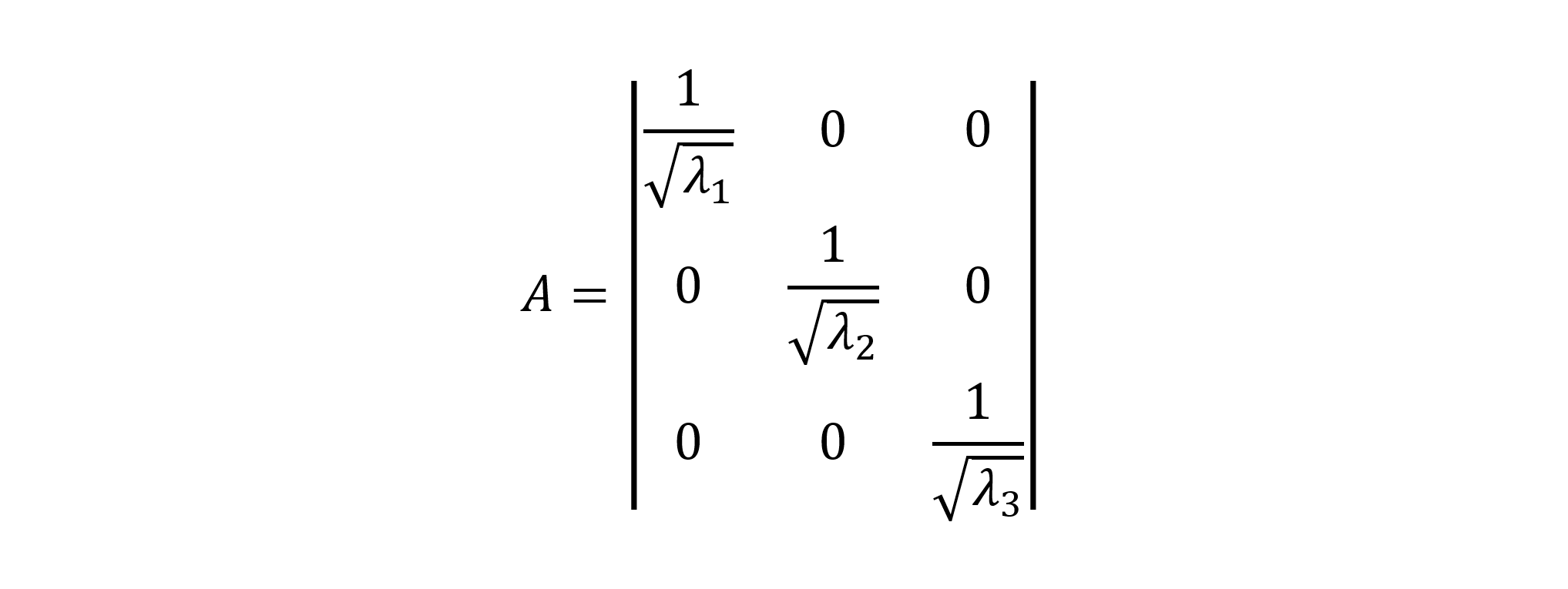
The SVD-decomposition algorithm solely relies on the matrix QR-decomposition, which yields obtaining the diagonal eigenvalues matrix E, as well as the matrix Ѵ of corresponding eigenvectors of A. The specific methods for the A's eigenvalues and eigenvectors computation have been previously discussed, above. To compute the diagonal singular values matrix Σ, the square root of each eigenvalue eᵢ ∈ E, 𝒊=𝟏..𝒏 is taken and placed onto the matrix Σ's diagonal, obtaining an inverse matrix of Σ, as shown below:

Herein, all eigenvalues in Σ must also be arranged in the ascending order, starting at the largest eigenvalue, assigned to the first diagonal element s₁₁=max{eᵢ ∈ E}. The resultant inverse matrix Σ⁻¹ is obtained, dividing 1.0 by each diagonal element sᵢᵢ ∈ Σ, such as that:
Finally, all diagonal elements in the inverse matrix Σ⁻¹ become the singular values of AᵗA.
Since we've computed the matrix AᵗA's singular values matrix Σ=Σ⁻¹, we're proceeding with the left and right singular vectors computation, discussed in the paragraph, below.
Step #3: Compute AᵗA's Right Singular Vectors:
The right singular vectors of AᵗA are normally obtained by finding a single non-trivial solution of the linear equation system, given both the eigenvalues diagonal vector e = diag{eᵢ ∈ E} and an identity matrix I with 1's at its diagonal:

The non-trivial solution of the linear equation system, above, is basically found by using the famous Jordan-Gaussian elimination approach, which yields the matrix AᵗA into the row echelon form reduction, and thus, the obtaining of an upper triangular matrix AᵗA.
Then, each of the right singular vectors is normalized by dividing all its components by the vector's absolute scalar length L, by using the following formula:

After that, the right singular vectors vᵢ ∈ V, 𝒊=𝟏..m are placed along the corresponding rows of the matrix V, and V is transposed, so that Vᵗ is finally a matrix of the right singular vectors of the matrix A.
Step #4: Compute AᵗA's Left Singular Vectors:
Since we've computed the matrices of singular values Σ and Vᵗ, now we can compute the A's left singular vectors matrix U, which is normally done by obtaining the product of the matrices A, Vᵗ and the diagonal Σ, such as:

The following computation results in obtaining A's left singular vectors matrix U, all singular vectors of which are the columns in U.
Finally, let's perform the verification of whether the A's SVD-decomposition has been done properly. Similar to the QR-decomposition, this is done by obtaining the product of U, Σ, and Vᵗ, which always must be approximately equal to the given matrix A.
The process of solving the singular value decomposition (SVD), illustrating the specific step-by-step SVD computations, has been thoroughly discussed in one of my previous articles "Singular Values Decomposition (SVD) In C++11 By An Example", Arthur V. Ratz, CodeProject, November 2018.
Modified Gram-Schmidt Orthogonalization
The Gram-Schmidt process, proposed in the mid-50s, was one of the first successful methods for the orthogonalization of real or complex matrices [1,4,5,6]. This is the easiest method to compute the QR-factorization of a given matrix. The other methods, such as the Householder reflections, based on the specular reflection, are typically even more complex. That's why let's briefly discuss the modified Gram-Schmidt orthogonalization method, first, and then, proceed with the Schwarz-Rutishauser algorithm explanation.
This method is primarily used for recursively finding matrices 𝑸 of 𝑨, based on the orthogonal projection of each vector 𝒂ₖ ∈ 𝑨, 𝒌=𝟏..𝒏 onto a span of already computed vectors 𝗾ᵢ ∈ 𝙌(𝒌), 𝒊=𝟏..𝒌. Each of the new orthogonal vectors 𝙦ₖ ∈ 𝙌 is computed as the sum of projections, subtracting each of the previously found orthogonal projections from a corresponding vector 𝒂ₖ ∈ 𝑨. Another, upper triangular matrix 𝑹 can be easily found as the product of 𝑸’s-transpose and the matrix 𝑨 using equation (1), above. According to the modified Gram-Schmidt method, the Gaussian elimination of each row of 𝑨 into 𝑹 is mostly done, in-place, while finding a corresponding column vector in 𝙌.
An orthogonal projection of 𝒂 onto 𝒒 is obtained by using the equation (2): below:

Normally, the modified Gram-Schmidt process yields the computation of matrix 𝙌 that can be algebraically expressed as:

, or alternatively:

Each new vector 𝙦ₖ ∈ 𝙌 is finally normalized by dividing it by its Euclidean norm |𝙦ₖ|.
A fragment of code in Python, listed below, implements the modified Gram-Schmidt orthogonalization process:
def conj_transpose(a):
    return np.conj(np.transpose(a))

def proj_ab(a,b):
    return a.dot(conj_transpose(b)) / lin.norm(b) * b

def qr_gs(A, type=complex):
    A = np.array(A, dtype=type)
    (m, n) = np.shape(A)

    (m, n) = (m, n) if m > n else (m, m)

    Q = np.zeros((m, n), dtype=type)
    R = np.zeros((m, n), dtype=type)

    for k in range(n):
        pr_sum = np.zeros(m, dtype=type)

        for j in range(k):
            pr_sum += proj_ab(A[:,k], Q[:,j])

        Q[:,k] = A[:,k] - pr_sum
        Q[:,k] = Q[:,k] / lin.norm(Q[:,k])

    if type == complex:
        R = conj_transpose(Q).dot(A)
    else: R = np.transpose(Q).dot(A)

    return -Q, -R
The modified Gram-Schmidt orthogonalization process has some disadvantages, such as numerical instability, as well as a notably high computational complexity, above 𝑶❨𝟐𝒎𝒏²❩, when applied to the large-sized matrices. Also, it requires a modification to determine a matrix’s leading dimension, when performing the decomposition of rectangular m-by-n matrices [4].
Schwarz-Rutishauser Algorithm
As you’ve probably have noticed, the Schwarz-Rutishauser algorithm, discussed, is entirely based on the modified Gram-Schmidt orthogonalization, which has a typically high complexity, caused by the computation of the orthogonal projection of each vector 𝒂ₖ ∈ 𝑨 onto vectors 𝗾ᵢ ∈ 𝙌(𝒌). And thus, we need a slightly different orthogonalization method, rather than computing multiple sums of the sums, done for each 𝒂ₖ vector's projection onto the span 𝙌(𝒌).
In this case, the complexity of the orthogonal projection operator is approximately - 𝑶❨𝟑𝒎❩. It negatively impacts the overall performance of the modified Gram-Schmidt process, itself [4]. The Schwarz-Rutishauser algorithm is applied as the modified Gram-Schmidt algorithm-level optimization.
Specifically, the Schwarz-Rutishauser algorithm is a modification of the modified Gram-Schmidt matrix orthogonalization method, proposed by H. R. Schwarz, H. Rutishauser and E. Stiefel, in their research work “Numerik symmetrischer Matrizen” (Stuttgart, 1968) [6]. The research, held, was motivated by the goal to reduce the complexity of the existing modified Gram-Schmidt projection-based method, improving its performance and numerical stability [5], over those popular reflections- and rotation-based methods.
The main idea behind the Schwarz-Rutishauser algorithm is that the 𝑨’s orthogonalization complexity can be drastically reduced, compared to the either modified Gram-Schmidt 𝑶❨𝟐𝒎𝒏²❩ or Householder 𝑶❨𝟐𝒎𝒏²-𝟬.𝟔𝒏³❩ methods [5].
To provide a better understanding of the Schwarz-Rutishauser algorithm, let’s take a closer look at the equation (2) and (3.1) from the right, shown above.
While computing the sum of 𝒂’s projections onto the span 𝙌(𝒌) vectors, we must divide the scalar product of vectors <𝒂,𝒒> by the squared norm |𝙦ₖ|² to normalize their product [2]. However, it’s not necessary, since each vector 𝗾ᵢ ∈ 𝙌(𝒌) has been already normalized at one of the previous 𝒌-th algorithm’s steps.
Since then, the equation (3.1) can be simplified, eliminating the division of the sum of projections by the squared norm [5], in the equation from the right, below:

Since 𝑹 is the inner product of 𝑸’s-transpose and 𝑨, then we can easily compute the 𝒊-th element of each column vector 𝒓ₖ as:

Herein, the scalar product of 𝗾ᵢ- and 𝒂ₖ-vectors is multiplied by the unit basis vector 𝙚ₖ of the corresponding hyperplane in Hilbert’s ambient space ℋ [2].
Then, let’s substitute the equation (4.2) to (4.1), and we'll finally have:

Since we admit that 𝑸 must be initially equal to 𝑨 (𝑸 =𝑨), the computation of vectors 𝗾 and 𝒓 can be done recursively, by using equations (4.2) and (4.3), above [5]:

According to the vector arithmetics, to get each new 𝒌-th column vector 𝙦ₖ ∈ 𝙌, we subtract the product of the span of previous vectors 𝗾ᵢ ∈ 𝙌(𝒌) and 𝒓ᵢₖ from the current vector 𝙦ₖ, which is also called the rejection of 𝒂ₖ. Let’s remind that 𝙦ₖ is a vector, that initially equals to the original vector 𝒂ₖ (𝙦ₖ=𝒂ₖ), and the sum operator can be finally wiped away from the equation (4.3).
In this case, we also need to compute 𝒓ₖₖ, which is the 𝒌-th diagonal element in 𝑹, the norm of |𝙦ₖ|:

, normalizing the new 𝒌-th column vector 𝙦ₖ ∈ 𝙌, dividing it by its norm, equal to the current diagonal element 𝒓ₖₖ, from the preceding step [5].
Finally, we can briefly formulate the Schwarz-Rutishauser algorithm:
1. Initialize matrix 𝙌, equal to 𝑨 (𝙌=𝑨), and 𝑹 as the matrix of 0s;
2. For each 𝒌-th column vector 𝙦ₖ ∈ 𝙌, 𝒌=𝟏..𝒏, do the following:
2.1. For the span of vectors 𝗾ᵢ ∈ 𝙌(𝒌), 𝒊=𝟏..𝒌, that are already known:
- Get the 𝒊-th element 𝒓ᵢₖ of the 𝒌-th column vector 𝒓ₖ ∈ 𝑹, equation (5.1);
- Update the 𝒌-th column vector 𝙦ₖ ∈ 𝙌, equation (5.2);
2.2. Proceed with the previous step 2.1, to orthogonalize vector 𝙦ₖ, and obtain the 𝒌-th column vector 𝒓ₖ;
3. Compute the diagonal element 𝒓ₖₖ as the 𝙦ₖ-vector’s norm 𝒓ₖₖ=|𝙦ₖ|, equation (5.3);
4. Normalize the 𝒌-th column vector 𝙦ₖ ∈ 𝙌, dividing it by its norm, equal to 𝒓ₖₖ from the previous step 3;
5. Proceed with the orthogonalization of 𝑨, performed in the steps 1–4, to compute the 𝑨’ orthonormal basis 𝙌 and the upper triangular matrix 𝑹;
6. Once done, return the negative resultant matrices -𝙌 and -𝑹 from the procedure;
As you can see from the fragment of code, below, the implementation of the Schwarz-Rutishauser algorithm has been drastically simplified, compared to the modified Gram-Schmidt process. Moreover, it provides an ability to simultaneously compute those vectors of matrices 𝑹 and 𝙌, in-place [5].
A fragment of the code, demonstrating an implementation of the Schwarz-Rutishauser algorithm is listed below:
def qr_gs_modsr(A, type=complex):

    A = np.array(A, dtype=type)
    (m,n) = np.shape(A)

    Q = np.array(A, dtype=type)
    R = np.zeros((n, n), dtype=type)

    for k in range(n):
        for i in range(k):
            R[i,k] = np.transpose(Q[:,i]).dot(Q[:,k]);
            Q[:,k] = Q[:,k] - R[i,k] * Q[:,i];

        R[k,k] = lin.norm(Q[:,k]); Q[:,k] = Q[:,k] / R[k,k];

    return -Q, -R
Numerical Stability and Complexity
Here're some of the potential issues with the Householder reflections or modified Gram-Schmidt orthogonalization methods, increasing the complexity, and thus, negatively impacting their performance:
- The complex conjugate transpose computation.
- The column-by-column sum of orthogonal projections computation.
- The new upper-triangular matrix R computation as the inner product of H and previous R.
Obtaining the householder matrix is mainly based on the specular reflection of each column vector in A, which yields the rotation of each vector by the 90° degree angle to find an orthonormal basis of A. In the complex matrix case, the complex conjugate transpose computation is required. The complex conjugate transpose operation has a larger complexity, compared to the entire modified Gram-Schmidt orthogonalization method. Thus, the complexity of the Householder reflections method is normally by O(n) - times greater while performing the decomposition of non-real large-sized matrices.
The overall complexity of the Householder reflections differs mostly by O(-0.6n³) - O(-0.6n⁴), compared to the modified Gram-Schmidt orthogonalization method's complexity, although does not always provide a sufficient performance speed-up on the large-sized matrices of the real type.
Both the Householder reflections and modified Gram-Schmidt orthogonalization methods have a different complexity in either real or complex matrix cases, proportional to either O(2mn²) or O(2mn³). The complexity of non-real matrix decomposition is n-times greater in the columns dimension, caused by the complex conjugate transpose computation.
Let’s take a look into the Schwarz-Rutishauser algorithm’s complexity. In most cases, it evaluates to 𝑶(𝙢𝙣²) and is constantly reduced at least as twice (2x) for both real and complex matrix cases [4,5].
The complexity of all three QR-decomposition algorithms is shown in the chart, below:

The Schwarz-Rutishauser and other QR-decomposition algorithms estimated complexity survey is visualized in the comparison chart, below:

As you can see, the overall complexity of the Schwarz-Rutishauser algorithm (navy) has been reduced by almost 61%, compared to the Householder reflections (red), and by 50% - compared to the modified Gram-Schmidt orthogonalization process (green).
An execution time of the specific codes, implementing the different QR-decomposition algorithms, discussed, is shown in the chart, below:
Matrix A (848 x 931):

In this case, the execution time of codes, implementing the various QR-algorithms was empirically assessed by performing the QR decomposition of two randomly generated matrices A of an arbitrary shape (848 x 931), in the real and complex cases. In the real case, the Householder reflections algorithm provides the best execution wall-time, and thus, the sufficient performance speed-up, compared to the orthogonalization-based methods.
Despite this, in the complex matrix case, the Schwarz-Rutishauser algorithm provides the best execution time, which is 2.33x times faster than the Householder reflections and 1.27x times faster, - than the modified Gram-Schmidt orthogonalization.
Numerical stability is another factor, having an impact on the QR decomposition efficiency. In many cases, approximating the highest precision floating-point values incurs the numerical instability issue caused by the persistent rounding error and arithmetic overflow [1]. Mostly, it largely depends on the matrix values numerical representation (e.g., real or complex), as well as the matrix shape and its values quantity. Mostly, the arithmetic overflow is incurred as the result of real values multiplication, exponentially increasing the number of digits, followed by the decimal point of the resultant floating-point value. In turn, the division of two real values causes the floating-point value simplification, which is a decreased number of decimal digits. It normally leads to a persistent precision loss issue.
According to the best practices, to avoid the significant precision loss while performing the QR decomposition, it’s recommended to represent the elements as rational numbers, based on using a vast of the existing multi-precision libraries (such as the mpmath or GMPY) for Python, Node.js and other programming languages, supporting the high-precision floating-point arithmetic functionality.
Using the Code
As I've already discussed, the following project includes the specific codes in Anaconda Python 3.8 and the latest NumPy library, implementing all three QR-decomposition methods, introduced in this article. First, I've developed a code, implementing the Householder reflections algorithm. Compared to the modified Gram-Schmidt and Schwarz-Rutishauser, an implementation of the Householder reflections is much more "heavy", rather than both of these methods. It's mainly based on the implementation of different procedures to compute the Householder matrix, for either real or complex matrix cases, respectively. Also, in the complex case, the following code must compute a matrix's conjugate transpose and determine the leading dimension for rectangular matrices. A code in Python, implementing the Householder reflections algorithm is listed below:
qr_hh_solver.py
#----------------------------------------------------------------------------
#   QR Factorization Using Householder Reflections v.0.0.1
#
#        Q,R = qr_householder(A)
#
#        The worst-case complexity of full matrix Q factorization:
#
#              In real case:   p = O(7MN^2 + 4N)
#              In complex case p = O(7MN^2 + 2(4MN + N^2))
#
#              An Example: M = 10^3, N = 10^2, p ~= 7.0 x 1e+9  (real)
#                          M = 10^3, N = 10^2, p ~= 7.82 x 1e+9 (complex)
#
#   GNU Public License (C) 2021 Arthur V. Ratz
#----------------------------------------------------------------------------

import numpy as np
import numpy.linalg as lin

def qr_hh(A, type=complex):

    (m,n) = np.shape(A) # Get matrix A's shape m - # of rows, m - # of columns

    cols = max(m, n) if m > n else min(m, n) # Determine the A's leading dimension:

                                             # Since we want Q - a square (cols x cols),
                                             # and R - a rectangular matrix (m x n),
                                             # the dimension must satisfy
                                             # the following condition:

                                             # if m > n, then take a maximum value in
                                             # (m,n) tuple
                                             # if m <= n, then take a minimum value in
                                             # (m,n) tuple

    # Q - an orthogonal matrix of m-column vectors
    # R - an upper triangular matrix (the Gaussian elimination of A to the row-echelon form)

    # Initialization: [ R - a given real or complex matrix A (R = A)                    ]
    #                 [ E - matrix of unit vectors (m x n), I - identity matrix (m x m) ]
    #                 [ Q - orthogonal matrix of basis unit vectors (cols x cols)       ]

    E = np.eye(m, n, dtype=type)
    I = np.eye(m, m, dtype=type)

    Q = np.eye(cols, cols, dtype=type)
    R = np.array(A, dtype=type)

    # **** Objective ****:

    # For each column vector r[k] in R:
       # Compute the Householder matrix H (the rotation matrix);
       # Reflect each vector in A through
       # its corresponding hyperplane to get Q and R (in-place);

    # Take the minimum in tuple (m,n) as the leading matrix A's dimension

    for k in range(min(m, n)):

        nsigx = -np.sign(R[k,k])                   # Get the sign of
                                                   # k-th diagonal element r[k,k] in R
        r_norm = lin.norm(R[k:m,k])                # Get the Euclidean norm of the
                                                   # k-th column vector r[k]

        u = R[k:m,k] - nsigx * r_norm * E[k:m,k]   # Compute the r[k]'s surface normal u
                                                   # as k-th hyperplane
                                                   # r_norm * E[k:m,k] subtracted from
                                                   # the k-th column vector r[k]

        v = u / lin.norm(u);                       # Compute v, |v| = 1 as the vector u
                                                   # divided by its norm

        w = 1.0                                    # Define scalar w,
                                                   # which is initially equal to 1.0

        # In complex case:

        if type == complex:

            # **** Compute the complex Householder matrix H ****

            v_hh = np.conj(v)                               # Take the vector v's complex
                                                            # conjugate
            r_hh = np.conj(R[k:m,k])                        # Take the vector r[k]'s
                                                            # complex conjugate

            w = r_hh.dot(v) / v_hh.dot(R[k:m,k])            # Get the scalar w as the
                                                            # division of vector
                                                            # products r_hh and v,
                                                            # v_hh and r[k], respectively

            # **** Compute the real Householder matrix H ****

            H = I[k:m,k:m] - (1.0 + w) * np.outer(v, v_hh)  # Compute the Householder
                                                            # matrix as the outer product of
                                                            # v and its complex conjugate
                                                            # multiplied by scalar 1.0 + w ,
                                                            # subtracted from the identity
                                                            # matrix I of shape (k..m x k..m)

            # **** Compute the complex orthogonal matrix Q ****

            Q_k = np.eye(cols, cols, dtype=type)            # Define the k-th square matrix
                                                            # Q_k of shape
                                                            # (cols x cols) as an identity
                                                            # matrix

            Q_k[k:cols,k:cols] = H;                         # Assign the matrix H to the
                                                            # minor Q_k of shape
            Q = Q.dot(np.conj(np.transpose(Q_k)))           # [k..cols x k..cols],
                                                            # reducing the minor Q_k's
                                                            # transpose conjugate to the
                                                            # resultant matrix Q

        # In real case:

        else:
            # **** Compute the real Householder matrix H ****

            H = I[k:m,k:m] - (1.0 + w) * np.outer(v, v) # Compute the matrix H as the
                                                        # outer product of vector v,
                                                        # multiplied by the scalar (1.0 + w),
                                                        # subtracting it
                                                        # from the identity matrix I of shape
                                                        # (k..m x k..m)

            # **** Compute the real orthogonal matrix Q ****

            Q_kt = np.transpose(Q[k:cols,:])        # Get the new matrix Q = (Q'[k]^T*H)
                                                    # of shape (m-1 x n) as
            Q[k:cols,:] = np.transpose(Q_kt.dot(H)) # the product of the minor's
                                                    # Q'[k]-transpose and matrix H,
                                                    # where minor Q'[k] - a slice of
                                                    # matrix Q starting at the k-th row
                                                    # (elements of each column vector q[k]
                                                    # in Q, followed by the k-th element)
                                                    # Finally take the new matrix Q's-transpose

        # **** Compute the upper triangular matrix R ****

        R[k:m,k:n] = H.dot(R[k:m,k:n])              # Get the new matrix R of shape
                                                    # (m-1 x n-1) as
                                                    # the product of matrix H and the
                                                    # minor M'[k,k] <- R[k:m,k:n]

    if type != complex:
        Q = np.transpose(Q)                         # If not complex, get the
                                                    # Q's-transpose

    return Q, R                                     # Return the resultant matrices Q and R
Another code in Python, implementing the famous modified Gram-Schmidt orthogonalization algorithm, is shown below. In this case, the modified Gram-Schmidt orthogonalization algorithm's implementation has been reduced, and finally becomes more attractive, performing the same matrix QR decomposition in the lesser number of steps. Although, it still requires the functionality for either determining the leading dimension, in the rectangular matrix case or obtaining the complex conjugate transpose. Similar to the Householder reflections' implementation, above, it's still based on the implementation of the different fragments of code for either real or complex matrix decomposition. As well, the modified Gram-Schmidt implementation has somewhat lesser complexity.
qr_gs_solver.py
#---------------------------------------------------------------------------
#   QR Factorization Using Modified Gram-Schmidt Orthogonalization v.0.0.1
#
#        Q,R = qr_gram_schmidt(A)
#
#        The worst-case complexity of full matrix Q factorization:
#
#              In real case:   p = O(5MNlog2(N))
#              In complex case p = O(5MNlog2(2N) + 6MN)
#
#              An Example: M = 10^3, N = 10^2, p ~= 3.33 x 1e+10 (real)
#                          M = 10^3, N = 10^2, p ~= 3.82 x 1e+10 (complex)
#
#   GNU Public License (C) 2021 Arthur V. Ratz
#---------------------------------------------------------------------------

import numpy as np
import numpy.linalg as lin

# Function: conj_transpose(a) returns the conjugate transpose of vector b

def conj_transpose(a): # Takes the conjugate of complex vector a's-transpose
    return np.conj(np.transpose(a))

# Function: proj_ab(a,b) returns the projection of vector a onto vector b

def proj_ab(a,b): # Divides the product of <a,b> by the norm |b|
                  # and multiply the scalar by vector b:
                  # In real case:     <a,b> - the inner product of two real vectors
                  # In complex case:  <a,b> - the inner product of vector a and
                  # vector b's conjugate transpose
    return a.dot(conj_transpose(b)) / lin.norm(b) * b

def qr_gs(A, type=complex):

    A = np.array(A, dtype=type)

    (m, n) = np.shape(A) # Get matrix A's shape m - # of rows, m - # of columns

    (m, n) = (m, n) if m > n else (m, m)    # Determine the A's leading dimension:

                                            # The leading dimension must satisfy
                                            # the following condition:
                                            #
                                            # if m > n, then the shape remains unchanged,
                                            #  and Q,R - are rectangular matrices (m x n)
                                            #
                                            # if m <= n, then the shape of Q,R
                                            #            is changed to (m x m),
                                            #            and Q,R - are square matrices

    # Q - an orthogonal matrix of m-column vectors
    # R - an upper triangular matrix (the Gaussian elimination of A to the row-echelon form)

    # Initialization: [ Q - a multivector of shape (m x n) ]
    #                 [ R - a multivector of shape (m x n) ]

    Q = np.zeros((m, n), dtype=type) # Q - matrix of 0's
    R = np.zeros((m, n), dtype=type) # R - matrix of 0's

    # **** Objective: ****

    # For each column vector a[k] in A:
       # Compute the sum of a[k]'s projections onto a span of column vectors a[0..k]
       # Compute all column vectors q[k] of the orthogonal matrix Q

    # Finally: Compute the upper triangular matrix R of matrix A

    # Take n as the leading matrix A's dimension

    for k in range(n):

        pr_sum = np.zeros(m, dtype=type)       # Define the sum of projections vector pr_sum

        # For a span of column vectors q[0..k] in Q,
        # compute the sum f a[k]'s projections onto each vector q[0..k] in Q

        for j in range(k):
            pr_sum += proj_ab(A[:,k], Q[:,j])  # Get the projection of a[k] onto q[j],
                                               # and accumulate the result
                                               # to the vector pr_sum

        # **** Compute the orthogonal matrix Q ****

        Q[:,k] = A[:,k] - pr_sum               # Compute the new k-th column vector
                                               # q[k] in Q by
                                               # subtracting the sum of projections
                                               # from the column vector a[k]

        Q[:,k] = Q[:,k] / lin.norm(Q[:,k])     # Normalize the new k-th column vector
                                               # q[k] dividing it by its norm

    if type == complex:

        # **** Compute the complex upper triangular matrix R ****

        R = conj_transpose(Q).dot(A)           # Compute the matrix R as the product of Q's
                                               # transpose conjugate and matrix A (real case)

        # **** Compute the real upper triangular matrix R ****

    else: R = np.transpose(Q).dot(A)           # Compute the matrix R as the product of
                                               # Q's-transpose
                                               # and matrix A (complex case)

    return -Q, -R                              # Return the resultant negative matrices Q and R
Next, I've implemented the efficient Schwarz-Rutishauser algorithm. As you've noticed from the code, listed below, an entire implementation was significantly reduced since it's no longer necessary to implement separate codes for the decomposition of real and complex matrices. Unlike two previous QR-algorithm implementations, it allows to simultaneously obtain the matrices Q and R, performing the specific computations, in-place, rather than computing the inner product of Q's transpose and A. As well, it does not require the complex conjugate transpose computation, which allows to drastically decrease the complexity of large-sized matrices decomposition.
qr_gs_schwrt_solver.py
#-----------------------------------------------------------------------------------
#   QR Factorization Using Schwarz-Rutishauser Algorithm v.0.0.1
#
#        Q,R = qr_gram_schmidt_modsr(A)
#
#        The worst-case complexity of full matrix Q factorization:
#
#           In real & complex cases: p = O(MNlog2(4N^3)
#
#                   An Example: M = 10^3, N = 10^2, p = 2.19 x 1e+6
#
#   GNU Public License (C) 2021 Arthur V. Ratz
#-----------------------------------------------------------------------------------

import numpy as np
import numpy.linalg as lin

def qr_gs_modsr(A, type=complex):

    A = np.array(A, dtype=type)

    (m,n) = np.shape(A) # Get matrix A's shape m - # of rows, m - # of columns

    # Q - an orthogonal matrix of m-column vectors
    # R - an upper triangular matrix (the Gaussian elimination of A to the row-echelon form)

    # Initialization: [ Q - multivector Q = A of shape (m x n) ]
    #                 [ R - multivector of shape (n x n)       ]

    Q = np.array(A, dtype=type)      # Q - matrix A
    R = np.zeros((n, n), dtype=type) # R - matrix of 0's

    # **** Objective: ****

    # For each column vector r[k] in R:
       # Compute r[k,i] element in R, k-th column q[k] in Q;

    for k in range(n):
        # For a span of the previous column vectors q[0..k] in Q,
        # compute the R[i,k] element in R as the inner product of vectors q[i] and q[k],
        # compute k-th column vector q[k] as the product of scalar R[i,k] and i-th vector q[i],
        # subtracting it from the k-th column vector q[k] in Q
        for i in range(k):

            # **** Compute k-th column q[k] of Q and k-th row r[k] of R ****
            R[i,k] = np.transpose(Q[:,i]).dot(Q[:,k]);
            Q[:,k] = Q[:,k] - R[i,k] * Q[:,i];

        # Compute the r[k,k] pseudo-diagonal element in R
        # as the Euclidean norm of the k-th vector q[k] in Q,

        # Normalize the k-th vector q[k] in Q, dividing it by the norm r[k,k]
        R[k,k] = lin.norm(Q[:,k]); Q[:,k] = Q[:,k] / R[k,k];

    return -Q, -R  # Return the resultant negative matrices Q and R
Finally, I've implemented the eigendecomposition QR algorithm that performs the eigenvalues and eigenvectors of a square 'real' matrix A computation:
qr_eigen_solver.py
import math
import cmath
import numpy as np

import numpy.linalg as lin

def qr_eig_solver(A, n_iters, qr):

    # Do the simple QR-factorization to compute the 'real' eigenvalues of A
    E = qr_simple(A, n_iters, qr)

    # Solve the polinomial for each diagonal sub-matrix E'
    # to obtain the 'complex' eigenvalues of A
    E = qr_eig_vals_complex_rt(E)

    # Sort the eigenvalues in the ascending order
    E = np.flip(np.sort(E))

    # Compute the eigenvectors V of A, solving the linear equation system,
    # eliminating A to row-echelon form using the Jordan-Gaussian method
    V = qr_eig_vecs_complex_rt(A, E)

    return E, V                     # Return the resultant vector E and matrix V

def qr_simple(A, n_iters, qr):

    # Initialization: [ E - a square (n x n) matrix of eigenvalues E = A ]
    E = np.array(A, dtype=float)

    # Do n_iters x n - iterations to compute the 'real' eigenvalues of A:
    for i in range(np.shape(A)[1] * n_iters):
        Q,R = qr(E, float);                      # Solve the QR-decomposition of E at i-th iteration
        E = np.transpose(Q).dot(E).dot(Q)        # Compute the product of Q's-transpose, E and Q as the new matrix E

    return E                                     # Return the resultant matrix of 'real' eigenvalues E

def qr_eig_vals_complex_rt(E):

    n = np.shape(E)[1]                    # Get the number of columns in E

    if n >= 2:                            # Check if the number of columns is >= 2

        es = np.zeros(n, dtype=complex)   # Initialize the array of complex roots

        i = 0

        # For each diagonal element E[i][i], solve the i-th polynomial:
        while i < n - 1:

            # Calculate the sub-matrix E[i:i+1,i:i+1]'s diagonal elements mean
            mu = (E[i][i] + E[i+1][i+1]) / 2

            # Obtain the determinant of the sub-matrix E[i:i+1,i:i+1]
            det = E[i][i] * E[i+1][i+1] - E[i][i+1] * E[i+1][i]

            # Take the complex square root of mu^2, subtracting the determinant of E[i:i+1,i:i+1],
            # to solve the diagonal sub-matrix's of rank ^2 polynomial (i.e., quadratic equation)
            dt_root = cmath.sqrt(mu**2 - det)

            # Compute the eigenvalues e22 and 33, by subtracting the complex square root value
            # from the average of diagonal elements in the sub-matrix es[0:2,0:2],
            # and place them along the sub-matrix es[0:2,0:2]'s diagonal
            e1 = mu + dt_root; e2 = mu - dt_root

            # If e1 is complex, add e1 and e2 to the array es
            if np.iscomplex(e1):
               # If real parts of e1 and e2 are equal, conjugate e2
               if e1.real == e2.real:
                  e2 = np.conj(e2)

               # Append the pair of eigenvalues e1 and e2 to the array es
               es[i] = e1; es[i+1] = e2

               # Sort up the eigenvalues e1 and e2 in the ascending order
               if es[i] < es[i+1]:
                  es[[i]] = es[[i+1]]

               i = i + 1

            i = i + 1

    E = np.diag(E)                         # Extract 'real' eigenvalues from the E's diagonal

    # Combine two arrays E and es of the 'real' and 'complex' eigenvalues
    es = [E[i] if i in np.argwhere(es == 0)[:,0]
            else es[i] for i in range(n)]

    return es                              # Return the resultant array of eigenvalues

def rot_complex(val):

    # Rotate the val's 'real' part by the 90-degree angle, counter clockwise
    v_rr = val.real * math.cos(math.pi / 2) + val.imag * math.sin(math.pi / 2)
    # Rotate the val's 'imaginary' part by the 90-degree angle, counter clockwise
    v_ri = val.real * math.sin(math.pi / 2) + val.imag * math.cos(math.pi / 2)

    return v_rr + 1.j * v_ri        # Return the new orthogonal complex value in the space C'n

def qr_eig_vecs_complex_rt(A, E):

    (m,n) = np.shape(A)

    V = np.identity(n, dtype=complex)

    # Compute eigenvectors of A by solving the quadrant polynomial
    # ============================================================

    # Reduce the matrix A to the Jordan-Gaussian row-echelon form:
    #   For each eigenvalue e in E and column-vector in V do the following:
    for (e,z) in zip(E, range(m)):

        Av = np.array(A, dtype=complex)

        # Subtract the eigenvalue e from each diagonal element in Av
        #np.fill_diagonal(Av, np.array([ a - e for a in np.diag(Av)], dtype=complex))

        for j in range(m):
            Av[j][j] = Av[j][j] - e

        # For each i-th row in Av do the following:
        for i in range(m-1):

            # Get the i-th row's basis element alpha
            alpha = Av[i][i]

            # If alpha is not 0 or 1 divide each element in i-th row of Av
            # by the row's basis element alpha,to get 1 at the position of alpha
            if alpha != 0 and alpha != 1:
               #Av[i] = np.array([Av[i][j] / alpha for j in range(m)], dtype=complex)
               for j in range(m):
                   Av[i][j] = Av[i][j] / alpha

            # If alpha is already 0 (in 'rare' case), exchange i-th and (i+1)-th rows of Av
            Av[[i, i+1]] = Av[[i+1, i]] if alpha == 0 else Av[[i, i+1]]

            # For each row in Av, do the row-echelon elimination
            # This turns its basis element alpha into 0 of each column in Av
            for k in range(m):

                theta = Av[k][i]            # Get the diagonal element theta

                if i != k: # If is this *NOT* the current i-th row in Av (i != k), eleminate alpha for i-th row
                #Av[k,i:] = np.array([Av[k][j] - Av[i][j] * theta for j in range(i,m)], dtype=complex) if i != k else Av[k,i:]
                   for j in range(i,m):
                       Av[k][j] = Av[k][j] - Av[i][j] * theta

        # Since the last (m-1)-th column of Av is the current eigenvector in V
        # Copy the (m-1)-th row to z-th column of V, assigning 1.0 to its last (m-1)-th element
        V[:,z] = Av[:,m-1]; V[m-1][z] = 1.0

        # Obtain the Euclidean norm of z-th column in V
        nV = lin.norm(V[:,z])
        # Norm the z-th eigenvector in V by dividing each of its elements by the norm nV
        V[:,z] = np.array([v / nV for v in V[:,z]], dtype=complex)

        # If eigenvalue e is complex, rotate the corresponding
        # eigenvector counter clockwise by 90-degree angle
        V[:,z] = [rot_complex(v) for v in V[:,z]] if e.imag != 0 else V[:,z]

        z = z + 1

    return V
To evaluate the performance of all QR algorithms, being implemented, I've developed a demonstration app, the source code of which is listed below. An entire demo app's code generates the random real and complex matrices of an arbitrary shape. It performs the same QR decomposition, based on the Schwarz-Rutishauser algorithm, and sanity check whether the decomposition was done correctly. Then, it estimates the code execution wall-time for each QR algorithm to determine which implementation provides a better performance speed-up. At the end of its execution, the demo app outputs the performance summary report, displaying "winner" and "looser" QR-algorithm for matrices of both real and complex types:
qr_eigen_factorization.py
import math
import cmath
import time
import random

import pandas as pd

import numpy as np
import numpy.linalg as linalg

from qr_hh_solver import *
from qr_gs_solver import *
from qr_gs_schwrt_solver import *

from qr_eigen_solver import *

iter_max       = 30

mat_shape      = { 'min': 6,   'max': 32   }
mat_shape_perf = { 'min': 750, 'max': 950  }

qr_alg         = [ { 'alg': qr_gs,       'name': 'Gram-Schmidt       ' },
                   { 'alg': qr_gs_modsr, 'name': 'Schwarz-Rutishauser' },
                   { 'alg': qr_hh,       'name': 'Householder        ' } ]

mat_types      = [ 'real   ', 'complex' ]

checkup_status = [ 'failed', 'passed' ]

checkup_banner  = "\n[ Verification %s... ]"
stats_banner    = "%s Matrix A Statistics:\n"
qr_test_banner  = "\nQR Factorization Of A `%s` Matrix Using %s Algorithm:"
eig_test_banner = "\nEigenvalues And Eigenvectors <E,V> of A `%s` Real Matrix (%dx%d):"
survey_banner   = "Matrix: %s    WINS: [ %s : %d secs  ] LOOSES: [ %s : %d secs ]"
perf_stats      = "%s : [ type: `%s` exec_time: %d secs verification: %s ]"

app_banner     = "QR Factorization v.0.0.2 CPOL License (C) 2022 by Arthur V. Ratz"

# Function: perf(A, qr, type=complex) evaluates the qr factorization method's execution wall-time in nanoseconds,
#           returns the tuple of the resultant matrices Q,R and the execution time

def perf(A, qr, type=complex):
    t_d = time.time(); Q,R = qr(A, type); \
        return Q, R, (time.time() - t_d)

def rand_matrix(rows, cols, type=complex):
    np.set_printoptions(precision=8)
    if type == complex:
        return np.reshape(\
              np.random.uniform(1, 10, rows * cols) + \
              np.random.uniform(-10, 10, rows * cols) *  1j, (rows, cols))
    else: return np.reshape(10 * np.random.uniform(\
            0.01, 0.99, rows * cols), (rows, cols))

def print_array(arr, alias, type=complex):
    fmt = 'complexfloat' \
        if type == complex else 'float'
    np.set_printoptions(precision=3, \
        suppress=True, formatter=fmt)
    if isinstance(arr, complex):
        eps = np.finfo(complex).eps; tol = 100
        arr = [np.real(m) if np.imag(m)<tol*eps else m for m in arr]
        arr = [np.asscalar(np.real_if_close(m)) for m in arr]
    if len(np.shape(arr)) == 2:
        print("\nMatrix %s (%dx%d):" % \
            (alias, len(arr), len(arr[0])),"\n")
    else:
        print("\nVector %s (len = %d):" % \
            (alias, len(arr)),"\n")
    pd.set_option('precision', 3); \
        df = pd.DataFrame(arr)
    df = df.to_string(index=False).replace('j','i')
    print(df)

def check(M1, M2):
    v1 = np.reshape(M1,-1)
    v2 = np.reshape(M2,-1)
    if len(v1) != len(v2):
       return False
    else: return 0 == len(np.where(np.array(\
       [ format(c1, '.4g') == format(c2, '.4g') \
        for c1,c2 in zip(v1, v2) ]) == False)[0])

def logo():
    print(app_banner)
    print(''.join(['=' for p in range(len(app_banner))]))

def qr_demo(s, qr, type=complex):

    print("QR-Decomposition of Matrix A:")
    print("=============================")

    print(qr_test_banner % (\
        "Complex" if type == complex \
            else "Real", s.replace(' ', '')))

    rows = np.random.randint(\
        mat_shape['min'], mat_shape['max'])

    cols = np.random.randint(\
        mat_shape['min'], mat_shape['max'])

    A1 = rand_matrix(rows, cols, type); print_array(A1, "A1")

    Q,R,T = perf(A1, qr, type)

    status_qr = check(A1, Q.dot(R))

    print_array(Q, "Q", type)
    print_array(R, "R", type)

    print(checkup_banner % (checkup_status[status_qr]),"\n")

    if type == complex:
       return status_qr

    rows = min(rows, cols)

    print(eig_test_banner % ("Real", rows, rows))

    A2 = np.array(A1[:rows,:rows], dtype=type)

    E,V = qr_eig_solver(A2, iter_max, qr)

    print_array(E, "E")
    print_array(V, "V")

    return status_qr

def qr_perf():

    print ("\nPerformance Assessment:")
    print ("=======================================")

    rows = np.random.randint(\
        mat_shape_perf['min'], mat_shape_perf['max'])

    cols = np.random.randint(\
        mat_shape_perf['min'], mat_shape_perf['max'])

    d = np.random.randint(5)
    cols += d if random.uniform(0,1) > 0.5 else -d

    A = [ rand_matrix(rows, cols, float), \
          rand_matrix(rows, cols, complex) ]

    print ("\nMatrix A (%d x %d):" % (rows, cols))
    print ("============================\n")

    exec_time = np.zeros((len(mat_types), len(qr_alg)))
    survey = np.zeros((len(mat_types), 1), dtype=object)

    status = 0
    for s_j in range(len(mat_types)):
        for s_i in range(len(qr_alg)):
            qr, name = \
                qr_alg[s_i]['alg'], qr_alg[s_i]['name']; \
                Q, R, exec_time[s_j][s_i] = perf(A[s_j],   \
                    qr, float if s_j % len(mat_types) == 0 else complex); \
                status = checkup_status[check(A[s_j], Q.dot(R))]
            print(perf_stats % (name, mat_types[s_j].replace(' ','').lower(), \
                exec_time[s_j][s_i], status))

            if status == "failed": break

        if status == "failed":
           print_matrix(A[s_j], "A")
           print_matrix(Q, "Q")
           print_matrix(R, "R")

           print("\n*** FAILURE!!! ****\n")

           break

        wr_time, lr_time = \
            np.min(exec_time[s_j]), \
            np.max(exec_time[s_j])

        wi = np.where(exec_time[s_j] == wr_time)[0][0]
        li = np.where(exec_time[s_j] == lr_time)[0][0]

        s_w = qr_alg[wi]['name']; s_l = qr_alg[li]['name']

        survey[s_j] = { 'alg_w': s_w, 'tm_w': wr_time, \
                        'alg_l': s_l, 'tm_l': lr_time }

        print("\n")

    for s_j in range(len(mat_types)):
        print(survey_banner % (mat_types[s_j].lower(),
              survey[s_j][0]['alg_w'], survey[s_j][0]['tm_w'], \
              survey[s_j][0]['alg_l'], survey[s_j][0]['tm_l']))

def main():

    logo()

    np.random.seed(int(time.time()))

    status = 0
    for s_j in range(len(qr_alg)):
        for s_i in range(len(mat_types)):
            status = qr_demo(qr_alg[s_j]['name'], \
                qr_alg[s_j]['alg'], float if s_i % 2 else complex)
            if status == False: break

        if status == False:
           print("\n*** FAILURE!!! ****\n"); break

    qr_perf(); print("\n")

if __name__ == "__main__":
    main()
Points of Interest
In conclusion, the Schwarz-Rutishauser algorithm, introduced in this article, is extremely fast and efficient, applied for the large-sized real and complex matrices of an arbitrary shape, which size is far beyond of 𝟏𝟎³ elements at each dimension. The overall complexity of the Schwarz-Rutishauser algorithm is just 𝑶(𝙢𝙣²), which is 𝑶(𝒏)-times less, compared to the modified Gram-Schmidt process, and is very close to matrices inner product operation's complexity. Finally, it’s considered to have much better numerical stability and is attractive for parallelization, scaling the specific code execution, across multiple cores in the modern symmetric CPUs.
References
- “QR-Decomposition” — From Wikipedia, the free encyclopedia
- “Projection (Linear Algebra)”- From Wikipedia, the free encyclopedia
- “Factorization” — From Wikipedia, the free encyclopedia
- “ECE133A — Applied Numerical Computing (6. QR-Factorization)”, Prof. L. Vandenberghe, University of California, Los Angeles, USA, Fall, 2019
- “Algorithms for the QR-Decomposition” by Walter Gander, Seminar Fuer Angewandte Mathematik Eidgenoessische Technische Hochschule CH-8092 ZUERIC, April 1980
- “Numerik symmetrischer Matrizen”, H. R. Schwarz, H. Rutishauser and E. Stiefel, Stuttgart, 1968
- “Eigendecomposition of a matrix” — From Wikipedia, the free encyclopedia
- "Math 108b: Advanced Linear Algebra, Lecture 5: The Schur Decomposition", Padraic Bartlett, University of California, Santa Barbara, 2014
- "Solving large scale eigenvalue problems", Lecture 4, March 14, 2018: The QR algorithm, Peter Arbenz, Computer Science Department, ETH Zurich
- "Facts About Eigenvalues" By Dr. David Butler, The University of Adelaide, Australia
- "Eigenvalue-Polynomials", September 7, 2017, MIT, Massachusetts, USA
- "Complex Eigenvalues of Real Matrices", Alex Freire, Department of Mathematics, University of Tennessee, USA, 2005
- "Computing Eigenvalues and/or Eigenvectors; Part 2, The Power method and QR-algorithm", Tom Lyche Centre of Mathematics for Applications, Department of Informatics, University of Oslo, November 16, Norway, 2008
- "Eigenvectors, Eigenvalues and Orthogonality", RiskPrep.com, July 22, 2021
- “Reducing vibration using QR decomposition and unconstrained optimization for a multi-rotor aircraft”, Bechhoefer, Eric Robert, Simmonds Precision Products, Inc., United States(US) Patent USP2009037512463, Feb 16, 2005
- “The Netflix Prize and Singular Value Decomposition”, NJIT, CS301-Spring 2021
History
- 11th December, 2021 - Article "Can QR Decomposition Be Actually Faster? Schwarz-Rutishauser Algorithm" was published.
- 17th December, 2021 - Article's contents and representation of the basic ideas have been revised.
- 20th December, 2021 - QR-decomposition visualization example and performance optimization content were added.
- 27th December, 2021 - QR-algorithm for computing the real matrices eigenspace and solving the SVD was explained.