
Nimbus SDK: A Tiny Framework for C++ Real-Time Volumetric Cloud Rendering, Animation and Morphing
5.00/5 (42 votes)
A reusable Visual C++ framework for real-time volumetric cloud rendering, animation and morphing

Index
1. Introduction
2. Theoretical background
2.1 Ray-tracing, ray-casting and ray-marching
2.2 Volumetric rendering
2.3 Water vapour emulation
2.4 Pseudospheroids
3.1 Class diagram
3.2 How to create a Gaussian cumulus
3.2.1 The main function
3.2.2 The render function
3.2.3 Simulating wind
3.2.4 Result
3.4 Creating a morphing effect
3.4.1 Linear interpolation
3.4.2 The main function
3.4.3 The render function
3.4.4 Result
4. Benchmarks
5. Conclusions and limitations
6. Further reading and references
7. Extended licenses
8. Download and documentation
9. Demo Video
1. Introduction
This article is a review of my PhD thesis titled "High-Performance Algorithms for Real-Time GPGPU Volumetric Cloud Rendering from an Enhanced Physical-Math Abstraction Approach" presented at the National Distance Education University in Spain (UNED) in October 2019 with summa cum laude distinction. The aim of this article is to explain the main features of the Nimbus SDK developed during the research.
Real-time volumetric cloud rendering is a complex task for novel developers who lack the math/physics knowledge. It is also a challenge for conventional computers without advanced 3D hardware capabilities. For this reason, the current Nimbus SDK provides an efficient base framework for low-performance nVidia graphics devices such as the nVidia GT1030 and the nVidia GTX 1050.
This framework may be applied in computer games, virtual reality, outdoor landscapes for architectural design, flight simulators, environmental scientific applications, meteorology, etc.
In the first lines, I will explain the current state-of-the-art and computer graphics background to understand the main principles explained hereby. Finally, a complete description of the SDK usage will be presented and exemplarized.
2. Theoretical Background
2.1 Ray-Tracing, Ray-Casting and Ray-Marching
The SDK core is based on ray-tracing principles. Basically, the ray-tracing consists in launching straight lines (rays) from the camera view, where a frame buffer is located, to the target scene: typically spheres, cubes, etc. as illustrated in Figure 1.
|
|
| Figure 1. Ray-tracing lay-out.
|
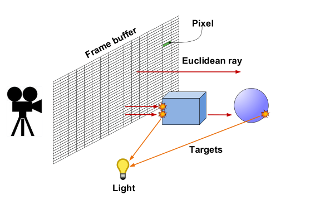
The math principle of the straight line is its Euclidean equation. The objective is to determine the collision of this line with the previously cited basic objects. Once the collisions have been determined, we can evaluate the color and other materials characteristics to produce the pixel color on the 2D frame buffer.
As ray-tracing is a brute force technique, other efficient solutions have been developed in the last decades. For example, in ray-casting methods, the intersections are analytically computed by using geometrical calculations. This approach is normally used along with other structures such as voxel grids and space partitioning algorithms. The method is usually applied in direct volume rendering for scientific and medical visualization to obtain a set of 2D slice images in magnetic resonance imaging (MRI) and computed tomography (CT).
In advanced real-time computer graphics, a widely used simplification of ray-tracing and ray-casting is known as raymarching. This method is a lightweight version of raycasting in which samples are taken down a line
in a discrete way to detect intersections with a 3D volume.
2.2 Volumetric Rendering
Many visual effects are volumetric in nature and are difficult to model with geometric primitives, including fluids, clouds, fire, smoke, fog and dust. Volume rendering is essential for medical and engineering applications that require visualization of three-dimensional data sets. There are two methods for volumetric rendering: Texture-based techniques and raycasting-based techniques. In texture-based volume rendering techniques perform the sampling and compositing steps by rendering a set of 2D geometric primitives inside the volume, as shown in Figure 2.
|
|
| Figure 2. View-aligned slicing with three sampling planes.
|

Each primitive is assigned texture coordinates for sampling the volume texture. The proxy geometry is rasterized and blended into the frame buffer in back-to-front or front-to-back order. In the fragment shading stage, the interpolated texture coordinates are used for a data texture lookup step. Then, the interpolated data values act as texture coordinates for a dependent lookup into the transfer function textures. Illumination techniques may modify the resulting color before it is sent to the compositing stage of the pipeline. [Iki+04].
In volume visualization with raycasting, high-quality images of solid objects are rendered which allows visualizing sampled functions of three dimensional spatial data like fluids or medical imaging. Most raycasting methods are based on Blinn/Kajiya models as illustrated in Figure 3.
Each point along the ray calculates the illumination I(t) from the light source. Let P be a phase function to compute the scattered light along the ray and D(t) be the local density of the volume. The illumination scattered along R from a distance t is:
where Θ is the angle between the view point and the light source.
The inclusion of the line integral from point (x,y,z) to the light source may be useful in applications where internal shadows are desired.
|
|
| Figure 3. A ray cast into a scalar function of a 3D volume.
|

The attenuation due to the density function along a ray can be calculated as Equation 2.
Finally, the intensity of the light arriving at the eye along direction R due to all the elements along the ray is defined in Equation 3:
intensive process, one or more of the following optimization processes are usually incorporated:
- Bounding boxes
- Hierarchical spatial enumeration (Octrees, Quadtrees, KD-Trees)
2.3 Water Vapour Emulation
To simulate water vapour droplets, a 3D noise texture is raymarched, as seen in Figure 4. We typically can use a Perlin noise or uniform random noise to generate fBm (fractal Brownian motion). The implementation of this SDK makes intensive use of the fBm noise as a summation of weighting uniform noise. Thus, let w be the octave scale factor, s the noise sampling factor and i the octave index, the fBm equation is defined as:
where w = 1/2 and s is 2.
|
|
| Figure 4. The uniform noise in the colour scale plot shows the irregular density of water droplets in a cloud raytraced hypertexture.
|

2.4 Pseudospheroids
One of the novel features provided by the Nimbus framework is the irregular realistic shape of clouds, thanks to the use of pseudospheroids. Basically, a pseudosphere is a sphere whose radius is modulated by a noise function as illustrated in Figure 5:
|
|
| Figure 5. Noise-modulated of a sphere radius.
|

The radius of the sphere follows Equation 5 during ray-marching:
(Eq. 5)
The Nimbus Framework
3.1 Class Diagram
The hyperlink below depicts the class diagram and the set of nineteen related classes and two interfaces of the SDK:

In the forthcoming sections, I will explain the usage of these classes step by step.
3.2 How to Create a Gaussian Cumulus
3.2.1 The Main Function
The class that creates a Gaussian cloud follows the density function of Equation 6:
(Eq.6)
It will typically generate a 3D plot similar to the one below:
|
|
| Figure 6. 3D Gaussian plot.
|

The code that creates the scene is shown below:
// Entry point for cumulus rendering
#ifdef CUMULUS

void main(int argc, char* argv[])
{
	// Initialize FreeGLUT and Glew
	initGL(argc, argv);
	initGLEW();

	try {
	    // Cameras setup
		cameraFrame.setProjectionRH(30.0f, SCR_W / SCR_H, 0.1f, 2000.0f);
		cameraAxis.setProjectionRH(30.0f, SCR_W / SCR_H, 0.1f, 2000.0f);
		cameraFrame.setViewport(0, 0, SCR_W, SCR_H);
		cameraFrame.setLookAt(glm::vec3(0, 0, -SCR_Z), glm::vec3(0, 0, SCR_Z));
		cameraFrame.translate(glm::vec3(-SCR_W / 2.0, -SCR_H / 2.0, -SCR_Z));

		userCameraPos = glm::vec3(0.0, 0.4, 0.0);

		// Create fragment shader canvas
		canvas.create(SCR_W, SCR_H);
		// Create cloud base texture
		nimbus::Cloud::createTexture(TEXTSIZ);

#ifdef MOUNT
		mountain.create(800.0, false); // Create mountain
#endif
		axis.create(); // Create 3D axis

		// Create cumulus clouds
		myCloud.create(35, 2.8f, glm::vec3(0.0, 5.0, 0.0), 0.0f, 3.0f,
                      0.0f, 1.9f, 0.0f, 3.0f, true, false);

		// Calculate guide points for cumulus
		myCloud.setGuidePoint(nimbus::Winds::EAST);

		// Load shaders
		// Main shader
		shaderCloud.loadShader(GL_VERTEX_SHADER, "../Nube/x64/data/shaders/canvasCloud.vert");
#ifdef MOUNT
		// Mountains shader for cumulus
		shaderCloud.loadShader(GL_FRAGMENT_SHADER,
       "../Nube/x64/data/shaders/clouds_CUMULUS_MOUNT.frag");
#endif
#ifdef SEA
		// Sea shader for cumulus
		shaderCloud.loadShader(GL_FRAGMENT_SHADER,
       "../Nube/x64/data/shaders/clouds_CUMULUS_SEA.frag");
#endif
		// Axis shaders
		shaderAxis.loadShader(GL_VERTEX_SHADER, "../Nube/x64/data/shaders/axis.vert");
		shaderAxis.loadShader(GL_FRAGMENT_SHADER, "../Nube/x64/data/shaders/axis.frag");

		// Create shader programs
		shaderCloud.createShaderProgram();
		shaderAxis.createShaderProgram();

#ifdef MOUNT
		mountain.getUniforms(shaderCloud);
#endif
		canvas.getUniforms(shaderCloud);
		nimbus::Cloud::getUniforms(shaderCloud);
		nimbus::Cumulus::getUniforms(shaderCloud);
		axis.getUniforms(shaderAxis);

		// Start main loop
		glutMainLoop();

	}
	catch (nimbus::NimbusException& exception)
	{
		exception.printError();
		system("pause");
	}

	// Free texture
	nimbus::Cloud::freeTexture();
}

#endif
Basically, the code above initializes the OpenGL and Glew libraries and locates the frame buffer and coordinate axis camera. After this, we define the cloud texture size, create the coordinate axis, the optional mountains and finally a Gaussian cumulus cloud with Cumulus::create(). Then we define the guide point for wind direction with the function Cumulus::setGuidePoint(windDirection). Before the rendering loop starts, we load and allocate the uniforms variables into the GLSL shader using Shader::loadShader(shader), Shader::createShaderProgram() and ::getUniforms() methods. Finally, we start the rendering loop. Do not forget to free textures by calling nimbus::Cloud::freeTexture() before closing down the application.
3.2.2 The Render Function
We have just initialized the OpenGL (FreeGLUT) , Glew and prepared a cumulus cloud. Then we tell FreeGLUT to draw the scene or display function that responds to wind advection and shadow precalculation. The implementation of this function is as follows:
#ifdef CUMULUS

// Render function
void displayGL()
{
	if (onPlay)
	{

		// Clear back-buffer
		glClear(GL_COLOR_BUFFER_BIT | GL_DEPTH_BUFFER_BIT);

		//////////////// CLOUDS ///////////////////

		// Change coordinate system
		glm::vec2 mouseScale = mousePos / glm::vec2(SCR_W, SCR_H);

		// Rotate camera
		glm::vec3 userCameraRotatePos = glm::vec3(sin(mouseScale.x*3.0),
                                       mouseScale.y, cos(mouseScale.x*3.0));

		glDisable(GL_DEPTH_TEST);

		shaderCloud.useProgram();
		if (firstPass) // If first iteration
		{

			// Render cloud base texture
			nimbus::Cloud::renderTexture();

#ifdef MOUNT
			// Render mountain
			mountain.render();

#endif
			nimbus::Cloud::renderFirstTime(SCR_W, SCR_H);
		}

			// Render cloud base class uniforms
			nimbus::Cloud::render(mousePos, timeDelta, cloudDepth,
                                 skyTurn, cloudDepth  * userCameraRotatePos, debug);

			// Calculate and apply wind
			(parallel) ? myCloud.computeWind(&windGridCUDA) :
                        myCloud.computeWind(&windGridCPU);

			// Wind setup
			nimbus::Cumulus::setWind(windDirection);

			// Render cumulus class
			nimbus::Cumulus::render(shaderCloud);

			if (precomputeTimeOut >= PRECOMPTIMEOUT) // Check for regular
                                                     // precompute light (shading)
			{
				clock_t start = clock();

				if (parallel)
				{
					if (skyTurn == 0)  // If morning sun is near else sun is far (sunset)
						nimbus::Cumulus::precomputeLight(precompCUDA, sunDir, 100.0f, 0.2f);
					else nimbus::Cumulus::precomputeLight
                                 (precompCUDA, sunDir, 10000.0f, 1e-6f);
					cudaDeviceSynchronize();
				}
				else
				{
					if (skyTurn == 0)
						nimbus::Cumulus::precomputeLight(precompCPU, sunDir, 100.0f, 0.2f);
					else nimbus::Cumulus::precomputeLight
                                          (precompCPU, sunDir, 10000.0f, 1e-6f);
				}
				clock_t end = clock();

				nimbus::Cloud::renderVoxelTexture(0);

				precomputeTimeOut = 0;
				float msElapsed = static_cast<float>(end - start);
				std::cout << "PRECOMPUTING LIGHT TIME ="
                         << msElapsed / CLOCKS_PER_SEC << std::endl;
			}

			if (totalTime > TOTALTIME)
			{
				timeDelta += nimbus::Cumulus::getTimeDir();
				totalTime = 0;
			}

			totalTime++;
			precomputeTimeOut++;

			// User camera setup
			cameraSky.setLookAt(cloudDepth * userCameraRotatePos, userCameraPos);
			cameraSky.translate(userCameraPos);

			canvas.render(cameraFrame, cameraSky);

			/////////////// AXIS ////////////////////

			shaderAxis.useProgram();

			// Render axis
			cameraAxis.setViewport(SCR_W / 3, SCR_H / 3, SCR_W, SCR_H);
			cameraAxis.setLookAt(10.0f * userCameraRotatePos, userCameraPos);
			cameraAxis.setPosition(userCameraPos);

			axis.render(cameraAxis);

			// Restore landscape viewport
			cameraFrame.setViewport(0, 0, SCR_W, SCR_H);

			glutSwapBuffers();

			glEnable(GL_DEPTH_TEST);
			//  Calculate FPS
			calculateFPS();
			firstPass = false; // First pass ended
	}
}

#endif
The first step of this function is updating the frame buffer camera and calculating the main scene camera that responds to mouse motion. This camera acts as a panning camera using mouse, but we can proceed to translate it by using the keypad arrows. We must start the rendering function with a call to the main Shader::useProgram(). In the first iteration, the following methods must be invoked: nimbus::Cloud::renderTexture(), optionally Mountain::render() and finally nimbus::Cloud::renderFirstTime(SCR_W, SCR_H) in this order. During the normal operation of the rendering loop, we must call to nimbus::Cloud::render() to pass values to the shader uniforms. Now, it is time to compute wind motion using the fluid engine with a call to: nimbus::Cumulus::setWind(windDirection)and Cumulus::computeWind() according to the device selection. The next step is precomputing shadows from time to time using nimbus::Cumulus::precomputeLight() using a specific precomputer object depending on whether the CPU or the GPU is selected. The last step is rendering their calculated textures by a call to nimbus::Cloud::renderVoxelTexture(cloudIndex) to render the shadow cloud texture.
3.2.3 Simulating Wind
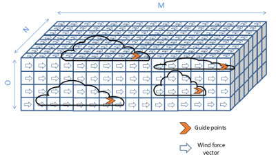
The NimbuSDK fluid engine is based on an internal 3D grid of U,V,W wind forces that acts over an automatic selected guide point for each cloud, as illustrated in Figure 7.
|
|
| Figure 7. Example of guide points inside a 3D fluid grid.
|
We will use the OpenGL(FreeGLUT) idle function to recalculate wind, as shown in the code below:
// Idle function
void idleGL()
{
	if (!onPlay) return;

	syncFPS();

#ifdef CUMULUS

	simcont++;
	if (simcont > FLUIDLIMIT) // Simulate fluid
	{
		applyWind();
		clock_t start = clock();
		if (parallel)
		{
			windGridCUDA.sendData();
			windGridCUDA.sim();
			windGridCUDA.receiveData();
			cudaDeviceSynchronize(); // For clock_t usage
		} else windGridCPU.sim();

		clock_t end = clock();
		float msElapsed = static_cast<float>(end - start);

		std::cout << "FLUID SIMULATION TIME = " << msElapsed / CLOCKS_PER_SEC << std::endl;
		simcont = 0;
	}
#endif
	glutPostRedisplay();
}
Basically, this idle function calls FluidCUDA::sendData() and FluidCUDA::sim() to send 3D grid data to the device before performing the simulation using CUDA. After the CUDA processing, a call to FluidCUDA::receiveData() is mandatory to retrieve the last processed fluid data. In the CPU case, it is not needed to send data to device, we must proceed to call FluidCPU::sim() directly.
#ifdef CUMULUS
void applyWind() // Apply wind force
{

	if (parallel)
	{
		windGridCUDA.clearUVW(); // Clear fluid internal data
		myCloud.applyWind(windForce, &windGridCUDA);
	} else
	{
		windGridCPU.clearUVW(); // Clear fluid internal data
		myCloud.applyWind(windForce, &windGridCPU);
	}

}
#endif
The code above must be called for the OpenGL idle function to apply wind to clouds.
3.2.4 Result
The previously explained code will result in the following image:
|
|
| Figure 8. A real-time cloud rendering.
|

3.3 Bounding Boxes
To avoid excessive tracing during raymarching, the framework wraps the different clouds inside marching cubes called bounding boxes. With this technique, it is possible to render high number of clouds by tracing the ones under the camera frustum and excluding all clouds behind and outside the camera view. This method is illustrated in Figure 9:
|
|
| Figure 9. Two rectangular bounding boxes with clouds processing a ray.
|

3.4 Creating a Morphing Effect
One of the most interesting features in the Nimbus SDK are the C++ classes related to cloud morphing effect. The implemented algorithm requires 90% decimation of 3D meshes before the animation loop, by using Blender or any other 3D commercial editor. The following sections explain the technical background to understand the algorithm basis.
3.4.1 Linear Interpolation
The transformation of two 3D wireframe meshes is performed by moving each pseudoellipsoid barycenter (i.e., the vertex) of the source shape to the target shape through linear interpolation as described in the following equation in GLSL:
(Eq.7)
where two situations may arise:
A) Barycenters in the source > Barycenters in the target mesh: In this case, we assign a direct correspondence between the barycenters in the source and target in iterative order. The excess barycenters in the source are randomly distributed by overlapping them across the target barycenters with the calculation of the modulus between their number of barycenters as seen in Figure 10.
|
|
| Figure 10. Case A. The excess barycenters in the hexagon are randomly distributed and overlapped over the triangle barycenters.
|

B) Barycenters in the target > Barycenters in the source mesh: The opposite operation implies a random reselection of the excess source barycenters to duplicate them and generate a new interpolation motion to the target mesh as seen in Figure 11.
|
|
| Figure 11. Case B. The required barycenters are added to the triangle for a random reselection to the hexagon barycenters.
|

3.4.2 The Main Function
// Entry point for mesh morphing
#ifdef MODEL

void main(int argc, char* argv[])
{
	// Initialize FreeGLUT and Glew
	initGL(argc, argv);
	initGLEW();

	try {
		// Cameras setup
		cameraFrame.setProjectionRH(30.0f, SCR_W / SCR_H, 0.1f, 2000.0f);
		cameraAxis.setProjectionRH(30.0f, SCR_W / SCR_H, 0.1f, 2000.0f);
		cameraFrame.setViewport(0, 0, SCR_W, SCR_H);
		cameraFrame.setLookAt(glm::vec3(0, 0, -SCR_Z), glm::vec3(0, 0, SCR_Z));
		cameraFrame.translate(glm::vec3(-SCR_W / 2.0, -SCR_H / 2.0, -SCR_Z));

		userCameraPos = glm::vec3(0.0, 0.4, 0.0);

		// Create fragment shader canvas
		canvas.create(SCR_W, SCR_H);
		// Create cloud base texture
		nimbus::Cloud::createTexture(TEXTSIZ);

#ifdef MOUNT
		mountain.create(300.0, false); // Create mountain
#endif
		axis.create(); // Create 3D axis
		model1.create(glm::vec3(-1.0, 7.0, 0.0), MESH1, 1.1f); // Create mesh 1
		model2.create(glm::vec3(1.0, 7.0, -3.0), MESH2, 1.1f);  // Create mesh 2
		morphing.setModels(&model1, &model2, EVOLUTE); // Setup modes for morphing

		// Load shaders
		// Main shader
		shaderCloud.loadShader
              (GL_VERTEX_SHADER, "../Nube/x64/data/shaders/canvasCloud.vert");
#ifdef MOUNT
		// Mountains shader for 3D meshes based clouds
		shaderCloud.loadShader(GL_FRAGMENT_SHADER,
              "../Nube/x64/data/shaders/clouds_MORPH_MOUNT.frag");
#endif
#ifdef SEA
		// Sea shader for 3D meshes based clouds
		shaderCloud.loadShader(GL_FRAGMENT_SHADER,
              "../Nube/x64/data/shaders/clouds_MORPH_SEA.frag");
#endif

		// Axis shaders
		shaderAxis.loadShader(GL_VERTEX_SHADER, "../Nube/x64/data/shaders/axis.vert");
		shaderAxis.loadShader(GL_FRAGMENT_SHADER, "../Nube/x64/data/shaders/axis.frag");

		// Create shader programs
		shaderCloud.createShaderProgram();
		shaderAxis.createShaderProgram();

		// Locate uniforms
		nimbus::Cloud::getUniforms(shaderCloud);

#ifdef MOUNT

		mountain.getUniforms(shaderCloud);

#endif

		canvas.getUniforms(shaderCloud);

		nimbus::Model::getUniforms(shaderCloud);

		axis.getUniforms(shaderAxis);

		// Start main loop
		glutMainLoop();

	}
	catch (nimbus::NimbusException& exception)
	{
		exception.printError();
		system("pause");
	}

	// Free texture
	nimbus::Cloud::freeTexture();
}

#endif
The initialization functions are the same as described for the cumulus section. It is also important to create the frame buffer canvas with Canvas::create() and the cloud texture by a call to nimbus::Cloud::createTexture(). Once this is made, we proceed to create the source and target mesh models with a call to Model::create() by passing the 3D position, the OBJ file path and the scale as arguments. Finally, we specify whether evolution (forwarding) or involution (backwarding) is preferred by a call to Morphing::setModels(). The rest of the code loads the GLSL shaders and locate the uniforms variables similarly as seen before.
3.4.3 The Render Function
#ifdef MODEL

void displayGL()
{
	if (onPlay)
	{

		// Clear back-buffer
		glClear(GL_COLOR_BUFFER_BIT | GL_DEPTH_BUFFER_BIT);

		// Change coordinate system
		glm::vec2 mouseScale = mousePos / glm::vec2(SCR_W, SCR_H);

		// Rotate camera
		glm::vec3 userCameraRotatePos =  glm::vec3(sin(mouseScale.x*3.0),
                                        mouseScale.y, cos(mouseScale.x*3.0));

		//////////////// MORPHING ///////////////////

		glDisable(GL_DEPTH_TEST);

		shaderCloud.useProgram();
		if (firstPass) // If first iteration
		{

			nimbus::Cloud::renderFirstTime(SCR_W, SCR_H);

			clock_t start = clock();
#ifdef CUDA
            // Precompute light for meshes
			nimbus::Model::precomputeLight(precompCUDA, sunDir,
                   100.0f, 1e-6f, model1.getNumEllipsoids(), model2.getNumEllipsoids());
#else
			nimbus::Model::precomputeLight(precompCPU, sunDir, 100.0f, 1e-6f,
                   model1.getNumEllipsoids(), model2.getNumEllipsoids());
#endif
			clock_t end = clock();
			std::cout << "PRECOMPUTE TIME LIGHT = " << end - start << std::endl;

			// Prepare for morphing
			(EVOLUTE) ? morphing.prepareMorphEvolute() : morphing.prepareMorphInvolute();
			alpha = alphaDir = 0.01f;
			// First morphing render
			nimbus::Model::renderFirstTime(model2.getNumEllipsoids(), EVOLUTE);

			// Render cloud base texture
			nimbus::Cloud::renderTexture();
#ifdef MOUNT
			// Render mountain
			mountain.render();
#endif

			// Render clouds precomputed light textures
			for (int i = 0; i < nimbus::Cloud::getNumClouds(); i++)
				nimbus::Cloud::renderVoxelTexture(i);
		}

		// Render cloud base class uniforms
		nimbus::Cloud::render(mousePos, timeDelta, cloudDepth, skyTurn,
                             cloudDepth * userCameraRotatePos, debug);

		static bool totalTimePass = false;

		if (totalTime > TOTALTIME) // Check time for morphing animation
		{
			totalTimePass = true;
			timeDelta += timeDir;
			if (alpha < 1.0 && alpha > 0.0)
			{
				alpha += alphaDir; // Animate morphing
				(EVOLUTE) ? morphing.morphEvolute(alpha) : morphing.morphInvolute(alpha);
				morphing.morph(0.1f); // Animation speed
			}

			totalTime = 0;
		}

		totalTime++;

		// Mesh renderer
		nimbus::Model::render(shaderCloud, (totalTimePass) ?
               morphing.getCloudPosRDst() : nimbus::Model::getCloudPosR(),
               morphing.getCloudPosDst(), alpha);


		// User camera setup
		cameraSky.setLookAt(cloudDepth * userCameraRotatePos, userCameraPos);
		cameraSky.translate(userCameraPos);

		canvas.render(cameraFrame, cameraSky);

		/////////////// AXIS ////////////////////

		shaderAxis.useProgram();

		// Render axis
		cameraAxis.setViewport(SCR_W / 3, SCR_H / 3, SCR_W, SCR_H);
		cameraAxis.setLookAt(10.0f * userCameraRotatePos, userCameraPos);
		cameraAxis.setPosition(userCameraPos);

		axis.render(cameraAxis);

		// Restore landscape viewport
		cameraFrame.setViewport(0, 0, SCR_W, SCR_H);

		glutSwapBuffers();

		glEnable(GL_DEPTH_TEST);
		//  Calculate FPS
		calculateFPS();
		firstPass = false; // First pass ended
	}
}

#endif
The main part of the OpenGL rendering function is similar to that seen in the cumulus section, so I will not insist on this. The essential difference lies in the function nimbus::Model::precomputeLight() that precomputates light only once. Then we have to call either Morph::prepareMorphEvolute() or Morph::prepareMorphInvolute() depending on the previously selected option. After initializing the linear interpolation variable counters: alpha for increment and alphaDir for positive or negative increment, we call nimbus::Model::renderFirstTime() with the number of the target ellipsoids and the preferred progression option. Before exiting the first pass iteration, it is required to call nimbus::Cloud::renderVoxelTexture(meshIndex) to pass the shadow voxel texture to the shader. Then, during the normal animation loop, we will proceed to feed the morphing effect with the corresponding calls to Morph::morphEvolute(alpha) or Morph::morphInvolute(alpha) depending on the selected option. As seen in the code above, it is straightforward to increment the animation counters often depending on the speed we need.
3.4.4 Result
Figures 12 to 18 to illustrate the morphing process of a hand into a rabbit:
|
|
|
| Figure 12. Step 1.
| Figure 13. Step 2.
|
|
|
|
| Figure 13. Step 3.
| Figure 14. Step 4.
|
|
|
|
| Figure 15. Step 5.
| Figure 16. Step 6.
|
|
|
|
| Figure 17. Step 7.
| Figure 18. Step 8.
|


4. Benchmarks
This section presents the benchmarks performed using GPU/CPU for nVidia GTX 1050 non-Ti (640 cores/Pascal) and GTX 1070 non-Ti (1920 cores/Pascal) under a 64-bit i-Core 7 CPU 860@2.80 GHz (first generation, 2009) with 6 GB RAM. The cumulus dynamic tests were performed over a moving sea scape with a real sky function using 4 clouds in the scene with 35 spheres each one (140 spheres in total). The benchmark versions were defined for each graphics card: a 103 precomputed light grid size with a 100 x 20 x 40 fluid volume and a 403 precomputed light grid size with a 100 x 40 x 40 fluid volume.
|
|
| Figure 19. 77.7 % of samples are above 30 FPS.
|

|
|
| Figure 20. 100% of samples are above 30 FPS.
|

|
|
| Figure 21. CUDA speed-up for light precomputation and fluid simulation in nVidia GTX 1050 non-Ti.
|

|
|
| Figure 22. CUDA speed-up for light precomputation and fluid simulation in nVidia GTX 1070 non-Ti.
|

5. Conclusions and Limitations
We can state that these algorithms are very good candidates for real-time cloud rendering with enhanced performance, thanks to atmospherical physical-math complexity abstraction and taking advantage of GPU/CPU multicore parallel technology to speed-up the computation. The Nimbus SDK v1.0 is in beta-stage, so some bugs might arise during your software operation. The main features of the framework are incomplete and they are susceptible of improvement, specially those that are able to be adapted for a better object-oriented programming and design patterns.
6. Further Reading and References
This article contents are extracted from my PhD thesis, that can be found at:
https://www.educacion.gob.es/teseo/mostrarRef.do?ref=1821765
and the following journal articles:
- Jiménez de Parga, C.; Gómez Palomo, S.R. Efficient Algorithms for Real-Time GPU Volumetric Cloud Rendering with Enhanced Geometry. Symmetry 2018, 10, 125. https://doi.org/10.3390/sym10040125 (*)
- Parallel Algorithms for Real-Time GPGPU Volumetric Cloud Dynamics and Morphing. Carlos Jiménez de Parga and Sebastián Rubén Gómez Palomo. Journal of Applied Computer Science & Mathematics. Issue 1/2019, Pages 25-30, ISSN: 2066-4273. https://doi.org/10.4316/JACSM.201901004
(*) If you find this work useful for your research, please, don't forget to cite the former reference in your journal paper.
Other references used in this article:
- [Iki+04] M. Ikits et al. GPU Gems. Addison-Wesley, 2004.
- [Paw97] J. Pawasauskas. “Volume Visualization With Ray Casting”. In: CS563 - Advanced Topics
in Computer Graphics Proceedings. Feb. 1997.
7. Extended Licenses
- Non physical based atmospheric scattering is CC BY-NC-SA 3.0 by robobo1221
- Elevated is CC BY-NC-SA by Iñigo Quilez
- Seascape is CC BY-NC-SA by Alexander Alekseev aka TDM
8. Download and Documentation
The API documentation and Visual C++ SDK are available for reading and download at: http://www.isometrica.net/thesis
and
https://github.com/maddanio/Nube