
Using Excel 2019 Features in Aspose.Cells
0/5 (0 vote)
In this article, I’ll demonstrate how to use Aspose.Cells to create a spreadsheet that takes advantage of a few new Excel 2019 features.
It’s no secret that working with Excel documents in .NET is notoriously tricky. In fact, back in the early days, it was downright tough. These days, .NET developers have a much easier job when it comes to generating, modifying, converting, or rendering spreadsheets. But even with modern components for manipulating spreadsheets at your disposal, getting your project completed can be difficult if the component you use doesn’t keep up with the latest Excel features.
With Aspose.Cells, creating spreadsheets is, quite frankly, a cakewalk, and the easy-to-use API now includes the ability to work with Excel 2019 formulas.
In this article, I’ll demonstrate how to use Aspose.Cells to create a spreadsheet that takes advantage of a few new Excel 2019 features. Some of the code I demonstrate might seem long-winded, but I want to be as clear as possible without obfuscating any logic.
Setting Up Your Project
The easiest way to start using Aspose.Cells is to use NuGet to download the required DLLs. I created a simple WinForms application that calls some code for creating the Excel document on a button click.
To add the NuGet package to your project, right-click on your solution and click Manage NuGet Packages. Search for "Aspose.Cells" and NuGet will display it as the first result. Now you can add the latest version of Aspose.Cells to your project.

Once NuGet has installed the packages, you’ll see the Aspose.Cells reference added to your project:

Now let’s start creating some spreadsheets.
The Complete Solution
The spreadsheet we’re going to create will use the following formulas:
- MAXIFS
- MINIFS
- IFS
- SWITCH
- CONCAT
- TEXTJOIN
The project will also illustrate how to add these charts to a spreadsheet:
- BoxWhisker
- Funnel
- ParetoLine
- Sunburst
- Treemap
- Waterfall
- Map
Let’s have a look at the formulas first.
We’ll create a spreadsheet that displays student scores for two semesters. Each score will receive a grade.
To display the grade, we’ll use the IFS formula.
Depending on the grade, we’ll use the SWITCH formula to display some text: Try harder, Ok, Good, Great or Excellent.
We’ll then use the CONCAT formula to concatenate the student name, grade, and text result.

Next we’ll display the highest and lowest scores for each semester. For this we’ll use the MAXIFS and MINIFS formulas.

Finally, we’ll use the TEXTJOIN formula to output the full name of each student, ignoring any blank cells.

Writing the Code
The first step is to add the required using statement:
using Aspose.Cells;
Next, we need to create a workbook and the path where the generated Excel document should be saved:
var wbook = new Workbook();
var pth = "C:/temp/aspose/";
Now create a method called SetupFormulaWorkbookData and pass it the worksheet, as follows:
private void SetupFormulaWorkbookData(Worksheet ws)
{
}
We’ll add code to this method in a minute. Let’s finish off the calling code first. Add a call to the SetupFormulaWorkbookData method and set the name of the worksheet to "Formulas". Then save the document in .xlsx format with the file name "1-Formulas.xlsx":
SetupFormulaWorkbookData(wbook.Worksheets[0]);
var ws = wbook.Worksheets[0];
ws.Name = "Formulas";
wbook.Save($"{pth}1-Formulas.xlsx", SaveFormat.Xlsx);
We need to write the code for the SetupFormulaWorkbookData method, but first we need to set up some data to work with. We’ll just hardcode these values for this example, but you could read data from a database or from a file.
Add the heading data needed:
ws.Cells["B2"].PutValue("Name");
ws.Cells["C2"].PutValue("Semester");
ws.Cells["D2"].PutValue("Score");
ws.Cells["E2"].PutValue("Grade");
Here are the hardcoded student names I used:
#region Add Names
ws.Cells["B3"].PutValue("John");
ws.Cells["B4"].PutValue("Lidia");
ws.Cells["B5"].PutValue("Mark");
ws.Cells["B6"].PutValue("Anne");
ws.Cells["B7"].PutValue("Hayley");
ws.Cells["B8"].PutValue("Lane");
ws.Cells["B9"].PutValue("Peter");
ws.Cells["B10"].PutValue("James");
ws.Cells["B11"].PutValue("Mary");
ws.Cells["B12"].PutValue("John");
ws.Cells["B13"].PutValue("Lidia");
ws.Cells["B14"].PutValue("Mark");
ws.Cells["B15"].PutValue("Anne");
ws.Cells["B16"].PutValue("Hayley");
ws.Cells["B17"].PutValue("Lane");
ws.Cells["B18"].PutValue("Peter");
ws.Cells["B19"].PutValue("James");
ws.Cells["B20"].PutValue("Mary");
#endregion
Next, add semesters 1 and 2 to the data:
#region Add Semesters
ws.Cells["C3"].PutValue(1);
ws.Cells["C4"].PutValue(2);
ws.Cells["C5"].PutValue(1);
ws.Cells["C6"].PutValue(2);
ws.Cells["C7"].PutValue(1);
ws.Cells["C8"].PutValue(1);
ws.Cells["C9"].PutValue(2);
ws.Cells["C10"].PutValue(1);
ws.Cells["C11"].PutValue(2);
ws.Cells["C12"].PutValue(2);
ws.Cells["C13"].PutValue(1);
ws.Cells["C14"].PutValue(2);
ws.Cells["C15"].PutValue(1);
ws.Cells["C16"].PutValue(2);
ws.Cells["C17"].PutValue(2);
ws.Cells["C18"].PutValue(1);
ws.Cells["C19"].PutValue(2);
ws.Cells["C20"].PutValue(1);
#endregion
Finally, add the student scores:.
#region Add Scores
ws.Cells["D3"].PutValue(75);
ws.Cells["D4"].PutValue(65);
ws.Cells["D5"].PutValue(15);
ws.Cells["D6"].PutValue(75);
ws.Cells["D7"].PutValue(95);
ws.Cells["D8"].PutValue(56);
ws.Cells["D9"].PutValue(72);
ws.Cells["D10"].PutValue(88);
ws.Cells["D11"].PutValue(24);
ws.Cells["D12"].PutValue(61);
ws.Cells["D13"].PutValue(72);
ws.Cells["D14"].PutValue(97);
ws.Cells["D15"].PutValue(17);
ws.Cells["D16"].PutValue(63);
ws.Cells["D17"].PutValue(84);
ws.Cells["D18"].PutValue(48);
ws.Cells["D19"].PutValue(65);
ws.Cells["D20"].PutValue(68);
#endregion
Of course, you can easily create this code using loops and reading the data from a file or database, but for simplicity sake, I just hardcoded the data.
The IFS Formula
We want to be able to display the grade of the student based on the score received, so we’ll use the IFS function.
Notice that in Excel you use a semicolon in the formula, but in Aspose.Cells, you need to use commas in the code instead of semicolons. To display the grades, we’ll loop through cells D3 to D20 and, if the cell value matches our condition, we’ll output a result of Fail, C, B, A or A+ in column E:
// IFS Formula
// eg: =IFS(D3<60;"Fail";D3<70;"C";D3<80;"B";D3<90;"A";D3>=90;"A+")
for (var i = 3; i <=20; i++)
{
    ws.Cells[$"E{i}"].Formula = $"=IFS(D{i}<60,\"Fail\",D{i}<70,\"C\",D{i}<80,\"B\",D{i}<90,\"A\",D{i}>=90,\"A +\")";
}
The SWITCH Formula
The same looping logic will be used to display some text based on the grade received. The text will be displayed in column F3 to F20 and will be based on the grades in column E3 to E20:
// SWITCH Formula
// eg: =SWITCH(E3;"Fail";"Try harder";"C";"Ok";"B";"Good";"A";"Great";"A+";"Excellent")
for (var i = 3; i <= 20; i++)
{
    ws.Cells[$"F{i}"].Formula = $"=SWITCH(E{i},\"Fail\",\"Try harder\",\"C\",\"Ok\",\"B\",\"Good\",\"A\",\"Great\",\"A +\",\"Excellent\")";
}
The CONCAT Formula
The CONCAT formula will use the name cells, the grade cells, and the text output to create a string that displays a message to the student. Again, we can use a loop to create the formula for each cell:
// CONCAT Formula
// eg: =CONCAT(B3;" - Result: "; E3; " - "; F3)
for (var i = 3; i <= 20; i++)
{
    ws.Cells[$"G{i}"].Formula = $"=CONCAT(B{i},\" - Your result: \", E{i}, \" - \", F{i})";
}
The MAXIFS and MINIFS Formulas
We now want to create the formulas to display the highest and lowest scores for each semester.
First, we need to add the header text and then the values for each semester as follows:
#region Results
ws.Cells["J2"].PutValue("Semester");
ws.Cells["K2"].PutValue("Highest");
ws.Cells["L2"].PutValue("Lowest");

ws.Cells["J3"].PutValue(1);
ws.Cells["J4"].PutValue(2);
#endregion
Next, we create the MAXIFS and MINIFS formulas for the highest and lowest cells for each semester:
var maxFirstSemesterCell = ws.Cells["K3"];
maxFirstSemesterCell.Formula = "=MAXIFS(D3:D20,C3:C20,\"1\")";

var maxSecondSemesterCell = ws.Cells["K4"];
maxSecondSemesterCell.Formula = "=MAXIFS(D3:D20,C3:C20,\"2\")";

var minFirstSemesterCell = ws.Cells["L3"];
minFirstSemesterCell.Formula = "=MINIFS(D3:D20,C3:C20,\"1\")";

var minSecondSemesterCell = ws.Cells["L4"];
minSecondSemesterCell.Formula = "=MINIFS(D3:D20,C3:C20,\"2\")";
The TEXTJOIN Formula
Finally, we want to generate full names for each student, including their first name, last name, and if they have it, a middle name. If they don’t have a middle name, the empty cell needs to be ignored.
Start by creating the data for the headings—the first, middle and last names:
#region Name Details
ws.Cells["B23"].PutValue("First name");
ws.Cells["C23"].PutValue("Middle name");
ws.Cells["D23"].PutValue("Last name");
ws.Cells["E23"].PutValue("Full name");

ws.Cells["B24"].PutValue("John");
ws.Cells["B25"].PutValue("Lidia");
ws.Cells["B26"].PutValue("Mark");
ws.Cells["B27"].PutValue("Anne");
ws.Cells["B28"].PutValue("Hayley");
ws.Cells["B29"].PutValue("Lane");
ws.Cells["B30"].PutValue("Peter");
ws.Cells["B31"].PutValue("James");
ws.Cells["B32"].PutValue("Mary");

ws.Cells["C24"].PutValue("Reginald");
ws.Cells["C27"].PutValue("Mary");
ws.Cells["C28"].PutValue("Lindy");
ws.Cells["C30"].PutValue("Lee");

ws.Cells["D24"].PutValue("Van Zandt");
ws.Cells["D25"].PutValue("Cunningham");
ws.Cells["D26"].PutValue("Lester");
ws.Cells["D27"].PutValue("Joseph");
ws.Cells["D28"].PutValue("Miller");
ws.Cells["D29"].PutValue("Bower");
ws.Cells["D30"].PutValue("Sanders");
ws.Cells["D31"].PutValue("Williams");
ws.Cells["D32"].PutValue("Davis");
#endregion
Now use another loop to create the full name for each student, ignoring any empty cells:
// TEXTJOIN Function
// eg: =TEXTJOIN(" "; TRUE; B24:D24)
for (var i = 24; i <= 32; i++)
{
    ws.Cells[$"E{i}"].Formula = $"=TEXTJOIN(\" \", TRUE, B{i}:D{i})";
}
Once you’ve set up all the data and formulas, running your application will generate an Excel document with the logic displayed earlier.
As you can see, creating Excel documents with formulas is very straightforward with Aspose.Cells.
Charts
Creating charts with Aspose.Cells is also pretty straightforward. What was traditionally a tricky process is much easier with Aspose.Cells. In fact, much of the same code can be used for the different charts.
We’ll create new Excel documents for each chart type. Let’s start off with a BoxWhisker chart.
The BoxWhisker Chart
The data we’ll use to generate the BoxWhisker chart is the volume of produce (Oranges, Apples, Pears and Grapes) for three years (2014, 2015 and 2016):

To use this data, start by creating a method called SetupBoxWhiskerChart that takes a Worksheet parameter:
private void SetupBoxWhiskerChart(Worksheet ws)
{
}
Next, create the headings for each column of data:
ws.Cells["B2"].PutValue("Produce");
ws.Cells["C2"].PutValue("Year 2014");
ws.Cells["D2"].PutValue("Year 2015");
ws.Cells["E2"].PutValue("Year 2016");
Now we’ll create the data for the produce (Oranges, Apples, Pears and Grapes). To do this, we’ll change things up a bit and use a loop with if statements to add each produce type four times (assume these are per term).
for (var i = 3; i <= 18; i++)
{
    if (i == 3 || i == 7 || i == 11 || i == 15)
        ws.Cells[$"B{i}"].PutValue("Oranges");

    if (i == 4 || i == 8 || i == 12 || i == 16)
        ws.Cells[$"B{i}"].PutValue("Apples");

    if (i == 5 || i == 9 || i == 13 || i == 17)
        ws.Cells[$"B{i}"].PutValue("Pears");

    if (i == 6 || i == 10 || i == 14 || i == 18)
        ws.Cells[$"B{i}"].PutValue("Grapes");
}
Next we’ll seed the year columns with random values for the amount produced in that year. For this, we’ll just use .NET’s built-in Random class. Note that if you require true random values, you need to create secure random numbers using RNGCryptoServiceProvider. We don’t require that level of randomness, so we’ll just use pseudo-random numbers.
var rnd = new Random();

for (var i = 3; i <= 18; i++)
{
    ws.Cells[$"C{i}"].PutValue(rnd.Next(10000, 70000));
    ws.Cells[$"D{i}"].PutValue(rnd.Next(10000, 70000));
    ws.Cells[$"E{i}"].PutValue(rnd.Next(10000, 70000));
}
Now we tell the worksheet which chart to create and then return the chartIndex for that chart. The values (6, 6, 25, 15) that follow ChartType.BoxWhisker specify the location of the chart in your Excel document.
var chartIndex = ws.Charts.Add(ChartType.BoxWhisker, 6, 6, 25, 15);
Add the series and category data to the chart. The series are each of the columns containing the volume data, and the category data defines the produce types (Oranges, Apples, Pears and Grapes).
var chart = ws.Charts[chartIndex];

_ = chart.NSeries.Add("=C3:C18", true);
_ = chart.NSeries.Add("=D3:D18", true);
_ = chart.NSeries.Add("=E3:E18", true);

chart.NSeries.CategoryData = "=B3:B18";
We now write our calling code:
var wbook = new Workbook();
var pth = "C:/temp/aspose/";
SetupBoxWhiskerChart(wbook.Worksheets[0]);
var ws = wbook.Worksheets[0];
ws.Name = "Charts";
wbook.Save($"{pth}2-BoxWhisker.xlsx", SaveFormat.Xlsx);
If you run the application now, you’ll see that the following BoxWhisker chart has been created:

That’s how easy it is to generate a chart in Aspose.Cells!
The Funnel Chart
Let’s mix things up a bit. Modify your SetupBoxWhiskerChart by renaming it to SetupChart and let it take an addition parameter of ChartType.
private void SetupChart(Worksheet ws, ChartType chrtType)
{
}
Now, keeping all the code exactly the same, just change the line that specifies the chart type and use the chrtType parameter passed into the method.
var chartIndex = ws.Charts.Add(chrtType, 6, 6, 25, 15);
If all is correct, your method should look as follows:
private void SetupChart(Worksheet ws, ChartType chrtType)
{
    ws.Cells["B2"].PutValue("Produce");
    ws.Cells["C2"].PutValue("Year 2014");
    ws.Cells["D2"].PutValue("Year 2015");
    ws.Cells["E2"].PutValue("Year 2016");

    for (var i = 3; i <= 18; i++)
    {
        if (i == 3 || i == 7 || i == 11 || i == 15)
            ws.Cells[$"B{i}"].PutValue("Oranges");

        if (i == 4 || i == 8 || i == 12 || i == 16)
            ws.Cells[$"B{i}"].PutValue("Apples");

        if (i == 5 || i == 9 || i == 13 || i == 17)
            ws.Cells[$"B{i}"].PutValue("Pears");

        if (i == 6 || i == 10 || i == 14 || i == 18)
            ws.Cells[$"B{i}"].PutValue("Grapes");
    }

    var rnd = new Random();

    for (var i = 3; i <= 18; i++)
    {
        ws.Cells[$"C{i}"].PutValue(rnd.Next(10000, 70000));
        ws.Cells[$"D{i}"].PutValue(rnd.Next(10000, 70000));
        ws.Cells[$"E{i}"].PutValue(rnd.Next(10000, 70000));
    }

    var chartIndex = ws.Charts.Add(chrtType, 6, 6, 25, 15);
    var chart = ws.Charts[chartIndex];

    _ = chart.NSeries.Add("=C3:C18", true);
    _ = chart.NSeries.Add("=D3:D18", true);
    _ = chart.NSeries.Add("=E3:E18", true);

    chart.NSeries.CategoryData = "=B3:B18";
}
Now you can modify your calling code slightly to create the workbook and set up the chart data, then pass it the chart type to generate. Rename the worksheet before saving the new Excel file.
var wbook = new Workbook();
var pth = "C:/temp/aspose/";
SetupChart(wbook.Worksheets[0], ChartType.Funnel);
var ws = wbook.Worksheets[0];
ws.Name = "Charts";
wbook.Save($"{pth}3-Funnel.xlsx", SaveFormat.Xlsx);
After creating the Excel document, open it and you’ll see the Funnel chart generated from the data for volume produce.

We can continue to create different charts using the exact same method, just changing the chart type passed to the method, as you’ll see below.
The ParetoLine Chart
Using the same method as before, let’s create a ParetoLine chart. Our calling code will change as follows:
SetupChart(wbook.Worksheets[0], ChartType.ParetoLine);
var ws = wbook.Worksheets[0];
ws.Name = "Charts";
wbook.Save($"{pth}4-Pareto.xlsx", SaveFormat.Xlsx);
This generates the following chart:
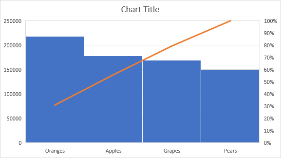
Again, the same method has generated a totally different chart type with minimal code changes.
The Sunburst Chart
The next chart type we’ll generate is the Sunburst. Modify the calling code as follows:
SetupChart(wbook.Worksheets[0], ChartType.Sunburst);
var ws = wbook.Worksheets[0];
ws.Name = "Charts";
wbook.Save($"{pth}5-Sunburst.xlsx", SaveFormat.Xlsx);
The resulting chart will be created in the saved Excel document and will look like this:

There are two more charts we’ll generate using our SetupChart method: the Treemap and Waterfall charts. I'm sure by this point you'll notice that the code needed to create the charts is simple and consistent. This makes it easy for you to set up code to accommodate whatever chart type your users might need.
The Treemap Chart
Modify the calling code as follows:
SetupChart(wbook.Worksheets[0], ChartType.Treemap);
var ws = wbook.Worksheets[0];
ws.Name = "Charts";
wbook.Save($"{pth}6-Treemap.xlsx", SaveFormat.Xlsx);
The Treemap chart, shown below, is created in the saved Excel document.

The Waterfall Chart
As before, modify the calling code to pass the Waterfall chart type:
SetupChart(wbook.Worksheets[0], ChartType.Waterfall);
var ws = wbook.Worksheets[0];
ws.Name = "Charts";
wbook.Save($"{pth}7-Waterfall.xlsx", SaveFormat.Xlsx);
The Waterfall chart, which looks like the following, is created in the saved Excel document.

The Map Chart
The last chart type we’ll look at is the Map chart. Here’s the data we’ll use to generate this chart:

First, create a method called SetupMapChart that takes a Worksheet as parameter:
private void SetupMapChart(Worksheet ws)
{
}
Next, create the column headings:
ws.Cells["B2"].PutValue("Country");
ws.Cells["C2"].PutValue("Sales");
Then add some countries under the Country heading:
ws.Cells[$"B3"].PutValue("South Africa");
ws.Cells[$"B4"].PutValue("Canada");
ws.Cells[$"B5"].PutValue("India");
ws.Cells[$"B6"].PutValue("France");
Again, we use the Random class to generate random sales volumes for each country. These random numbers will be between 50,000 and 70,000.
var rnd = new Random();

for (var i = 3; i <= 6; i++)
{
    ws.Cells[$"C{i}"].PutValue(rnd.Next(50000, 70000));
}
As before, create a chart type of Map and add the series and category data:
var chartIndex = ws.Charts.Add(ChartType.Map, 6, 6, 25, 15);
var chart = ws.Charts[chartIndex];

_ = chart.NSeries.Add("=C3:C6", true);

chart.NSeries.CategoryData = "=B3:B6";
Now call the SetupMapChart method and save the Excel document as follows:
SetupMapChart(wbook.Worksheets[0]);
var ws = wbook.Worksheets[0];
ws.Name = "Charts";
wbook.Save($"{pth}8-Map.xlsx", SaveFormat.Xlsx);
This will result in the following Map chart being generated.

You can see that the countries are highlighted in a darker shade of blue as the sales volumes increase. The lightest blue color indicates the lowest volume in sales.
Conclusion
This article only briefly touches on the different charts and formulas you can create using Aspose.Cells, and this is but a tiny part of what you can do using Aspose.Cells. To learn more about what Aspose.Cells can do for you, have a look at their web page.