Numerical Methods with C++ Part 4: Introduction Into Decomposition Methods of Linear Equation Systems

thoughts-on-coding

Rate me:

5.00/5 (2 votes)

3 Dec 2019CPOL12 min read

6.3K

Matrices are a key concept in solving linear equation systems. Efficient implementations of matrices are not only considering computation complexity but also space complexity of the matrix data.

Welcome back to a new post on thoughs-on-cpp.com. This time we will have a closer look at a possible implementation of a matrix and decomposition algorithms used for solving systems of linear equations. But before we dive deep into implementations of decomposition methods we first need to do a little excursion into the performance of different types of containers we could use to eventually store the data. As always you can find the respective repository at GitHub. So let’s have some fun with matrices.

Implementing a matrix

So let’s start by defining what we mean when we talk about matrices. Matrices are rectangular representations of the coefficients of linear equation systems of $N$ linear equations with $M$ unknowns such as

$\begin{matrix}2x+1.5y-3z = 2 \\1.2x-0.25y-1z = 3 \\0.5y+1.5z = 1\end{matrix}\rightarrow\begin{pmatrix}2 & 1.5 & -3 \\1.2 & -0.25 & -1 \\0 & 0.5 & 1.5\end{pmatrix}\begin{pmatrix}x \\y \\z\end{pmatrix}=\begin{pmatrix}2 \\3 \\1\end{pmatrix}$

A special subset of matrices are invertible matrices with $N$ linear equations and $N$ unknowns which we will discuss in this post. They are a key concept in linear algebra and used at almost every area in mathematics to represent linear transformations such as rotation of vectors in three-dimensional space. Knowing this a representation of the data as a two-dimensional vector would somehow feel natural not only because of the structure of the data but also how to access the data. As a result, the first rough implementation of a matrix could look like this

.gist table { margin-bottom: 0; }

A very simple matrix implementation

To get a simpler, and more natural, way to access the data, the implementation provides two overloads of the function call operator() (1,2) which are defining the matrix as a function object (functor). The two overloads of the function call operator() are necessary because we are not only want to manipulate the underlying data of the matrix but also want to be able to pass the matrix as a constant reference to other functions. The private AssertData() (3) class function guarantees that we only allow quadratic matrices. For comparison reasons, the matrix provides a ‘naive’ implementation of matrix multiplications realized with an overloaded operator*() (4) whose algorithm has a computational complexity of $O(n^3)$ . Real-life implementations of matrix multiplication are using Strassen’s algorithm, with a computational complexity of $\approx O(n^{ 2.807 })$ , or even more sophisticated algorithms. For our purpose, we only need the matrix multiplication to explore a little bit of the performance of the matrix implementation and verify the matrix decomposition methods.

Bound of Different Matrix Multiplication Algorithm — Bound of different matrix multiplication algorithm (Wikipedia)

Analysis of Performance

Until now we still don’t know if we really should use a two-dimensional vector, regarding computational performance, to represent the data or if it would be better to use another structure. From several other linear algebra libraries, such as LAPACK or Intel’s MKL, we might get the idea that the ‘naive’ approach of storing the data in a two-dimensional vector would be suboptimal. Instead, it is a good idea to store the data completely in one-dimensional structures, such as STL containers like std::vector or std::array or raw C arrays. To clarify this question we will examine the possibilities and test them with quick-bench.com.

Analysis of std::vector<T>

std::vector<T> is a container storing its data dynamic (1,2,3) on the heap so that the size of the container can be defined at runtime.

.gist table { margin-bottom: 0; }

Excerpt of the std::vector<T> implementation from libstdc++

The excerpt of the libstdc++ illustrates also the implementation of the access operator[] (4). And because the std::vector<T> is allocating the memory on the heap, the std::vector<T> has to resolve the data query via a pointer to the address of the data. This indirection over a pointer isn’t really a big deal concerning performance as illustrated at chapter heap-vs-stack further down the article. The real problem is evolving with a two-dimensional std::vector<T> at the matrix multiplication operator*() (5) where the access to the right hand side, rhs(j,k), is violating the row-major-order of C++. A possible solution could be to transpose the rhs matrix upfront or storing the complete data in a one-dimensional std::vector<T> with a slightly more advanced function call operator() which retrieves the data.

std::vector<T> is fulfilling the requirement of a ContiguousContainer which means that it’s storing its data in contiguous memory locations. Because of the contiguous memory locations, the std::vector<T> is a cache friendly (Locality of Reference) container which makes its usage fast. The example below illustrates the contiguous memory locations of a std::vector<int> with integer size of 4-byte.

.gist table { margin-bottom: 0; }

Example to show contiguous memory locations of a std::vector<int>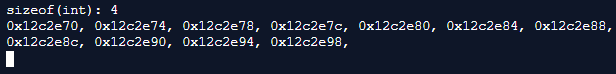

Contiguous memory locations of a std::vector with a 4 byte integer — Contiguous memory locations of a std::vector with a 4-byte integer

A slightly extended example with a two-dimensional array is pointing out the problem we will have, with this type of container, to store the matrix data. As soon as a std::vector<T> has more than one dimension it is violating the Locality of Reference principle, between the rows of the matrix, and therefore is not cache-friendly. This behavior is getting worse with every additional dimension added to the std::vector<T>.

.gist table { margin-bottom: 0; }

Multi-dimension std::vector<T> example

Multi-dimensional std::vector with a 4 byte integer and 24 byte row — Multi-dimensional std::vector with a 4-byte integer and 24-byte row

Analysis of std::array<T, size>

std::array<T, size> is a container storing its data on the stack. Because of the memory allocation on the stack, the size of std::array<T, size> needs to be defined at compile time. The excerpt of libstdc++ illustrates the implementation of std::array<T, size>. std::array<T, size> is in principle a convenience wrapper of a classical C array (1).

.gist table { margin-bottom: 0; }

Excerpt of the std::array<T, size> implementation from libstdc++

Heap vs. Stack

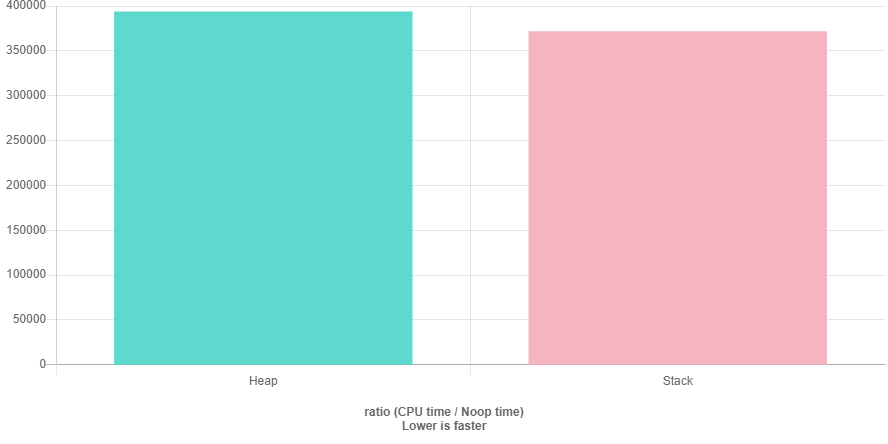
The code below shows a simple test of the performance difference between memory allocated on the heap and allocated on the stack. The difference can be explained by the fact that memory management on the heap needs an additional level of indirection, a pointer which points to the address in memory of the data element, which is slowing down the heap a little bit.

.gist table { margin-bottom: 0; }

Code used with quick-bench.com

Benchmark results with GCC-9.1 and O3 optimization of heap and stack (quick-bench.com)

Benchmarks

The code below is Benchmarking the 4 different ways to store the data (two- and one-dimensional std::vector, std::array, C array) and in addition shows the performance of a C array wrapped in std::unique_ptr<T[]>. All Benchmarks are done with Clang-8.0 and GCC-9.1.

.gist table { margin-bottom: 0; }

Code used with quick-bench.com

The graphs below point out what we already thought might happen, the performance of a two-dimensional std::vector is worse than the performance of a one-dimensional std::vector, std::array, C array, and the std::unique_ptr<T[]>. GCC seems to be a bit better (or more aggressive) in code optimization then Clang, but I’m not sure how comparable performance tests between GCC and Clang are with quick-bench.com.

Benchmark results with gcc-9.1 and O3 optimization (quick-bench.com)

Benchmark results with clang-8.0 and O3 optimization (quick-bench.com)

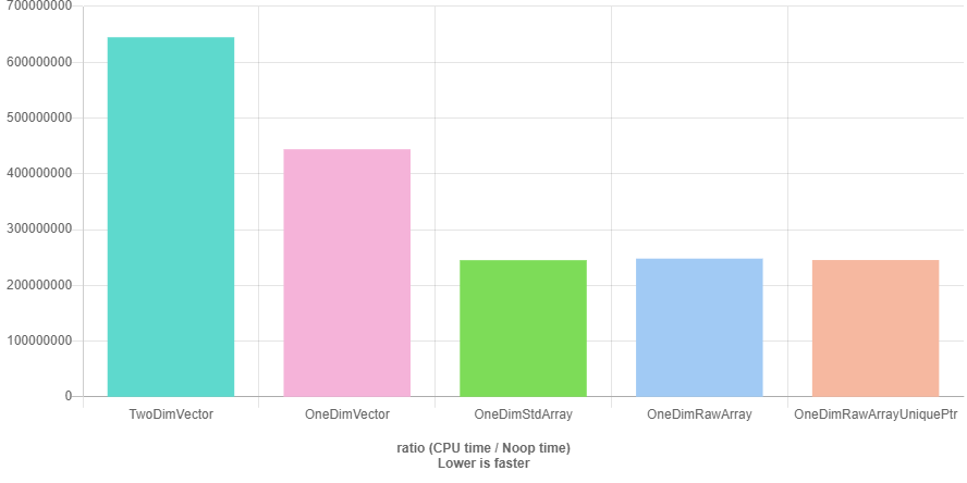
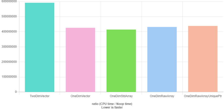
If we would choose Clang as compiler it wouldn’t make a difference if we would take a std::vector or one of the others, but for GCC it does. std::array we can’t choose because we want to define the size of the matrix at runtime and therefore std::array is not an option. For our further examination of a possible matrix implementation we could choose a C array, but for simplicity, safer memory management we will use std::unique_ptr<T[]>. std::vector<T> to store the data and querying the data via data() would also be an option.

Resulting Basis Matrix Implementation

.gist table { margin-bottom: 0; }

Resulting basis implementation of Matrix

Decomposition Methods

Let’s finally start discussing different matrix decomposition methods after all these preceding performance considerations.

LU-Decomposition

As long as we can guarantee that all main diagonal elements (also called pivot elements) are unequal to zero at any iteration of the decomposition $\left(a_{nn}^{(n-1)}\neq0\right)$ , we can use a simple LU-Decomposition.

$A=LU$

The LU-Decomposition (also known as Gaussian elimination) method is decomposing a given matrix A into two resulting matrices, the lower (L) matrix which contains quotients and main diagonal elements of value 1, and the upper (U) matrix which contains the resulting elements. Through back substitution, the upper matrix can be used to get the solution of the linear equation system.

$Ux=c$

At first (1) the main diagonal elements of the L matrix need to be initialized with 1. The quotients (2) of the L matrix can then be calculated by

$l_{ik}=\frac{a_{ik}^{(k-1)}}{a_{kk}^{(k-1)}}$

And the results (3) of the matrix U can afterward be calculated by

$r_{ik}=a_{ik}^{(i-1)}-l_{i,i-1}a_{i-1,k}^{(i-2)}$

.gist table { margin-bottom: 0; }

Implementation of LU-Decomposition

An example of a matrix A and its decomposition matrices L and U would look like the following.

$A=\begin{pmatrix}1 & 2 & 3 \\1 & 1 & 1 \\3 & 3 & 1\end{pmatrix}L=\begin{pmatrix}1 & 0 & 0 \\1 & 1 & 0 \\3 & 3 & 1\end{pmatrix}U=\begin{pmatrix}1 & 2 & 3 \\0 & -1 & -2 \\0 & 0 & -2\end{pmatrix}$

We have now a reliable algorithm to decompose an invertible matrix and solve the linear equation system. So let’s say we have one of these invertible matrices which have non zero main diagonal pivot elements. It should be no problem to solve the linear equation system with the algorithm described above, now. Let’s find out and say we have to solve the following linear equation system, with an accuracy of 5 digits, which should lead to the results $x_1=2.5354$ and $x_2=2.7863$ :

$\begin{pmatrix} 0.00035 & 1.2654 \\ 1.2547 & 1.3182 \end{pmatrix} \begin{pmatrix} x_1 \\ x_2 \end{pmatrix}=\begin{pmatrix} 3.5267 \\ 6.8541 \end{pmatrix}$

After solving the linear equation system we can get the results of $x_1$ and $x_2$ by back substitution

$x_2=\frac{-12636.0}{-4535.0}=2.7863$

$x_1=\frac{35267-1.2654 \cdot x_2}{0.00035}=\frac{3.5267-3.5258}{0.00035}=\frac{0.0009}{0.00035}=2.5714$

Unfortunately, the result of $x_1$ is quite off-target. The problem is the loss of significance due to the difference between the two values of the almost same size. To solve this problem we need the partial pivoting strategy which is exchanging the actual pivot element with the value of the largest element of the column. Ok let’s try again with the example above, but this time we have exchanged both rows to have the maximum values at the main diagonal pivots:

$\begin{pmatrix} 1.2547 & 1.3182 \\ 0.00035 & 1.2654 \end{pmatrix} \begin{pmatrix} x_1 \\ x_2 \end{pmatrix}=\begin{pmatrix} 6.8541 \\ 3.5267 \end{pmatrix}$

Again after solving the linear equation system we can get the results of $x_1$ and $x_2$ by back substitution

$x_2=\frac{3.5248}{1.2654}=2.7864$

$x_1=\frac{6.8541-1.3182\cdot x_2}{1.2547}=\frac{6.8541-3.6730}{1.2547}=\frac{3.1811}{1.2547}=2.5353$

Now the results are much better. But unfortunately, we can prove that also performing a partial pivoting, according to the largest element in the column, is not always sufficient. Let’s say we have the following linear equation system

$\begin{pmatrix} 2.1 & 2512 & -2516 \\ -1.3 & 8.8 & -7.6 \\ 0.9 & -6.2 & 4.6 \end{pmatrix} \begin{pmatrix} x_1 \\ x_2 \\ x_3 \end{pmatrix}=\begin{pmatrix} 6.5 \\ -5.3 \\ 2.9 \end{pmatrix}$

And after solving the linear equation system and applying partial pivoting before each iteration, the solution looks like

$\begin{pmatrix} 2.1 & 2512 & -2516 \\ 0 & 1563.9 & -1565.1\\ 0 & -1082.8 & 1082.9 \end{pmatrix} \begin{pmatrix} x_1 \\ x_2 \\ x_3 \end{pmatrix}=\begin{pmatrix} 6.5 \\ -1.2762 \\ 0.1143 \end{pmatrix}$

$\begin{pmatrix} 2.1 & 2512 & -2516 \\ 0 & 1563.9 & -1565.1\\ 0 & 0 & -0.7 \end{pmatrix} \begin{pmatrix} x_1 \\ x_2 \\ x_3 \end{pmatrix}=\begin{pmatrix} 6.5 \\ -1.2762 \\ -0.76930 \end{pmatrix}$

As a result, after the back substitution, we get $x_1=5.1905$ and $x_2=x_3=1.0990$ , but the exact results are $x_1=5$ and $x_2=x_3=1$ . Again the solution if off-target. The difference of the exact and numerical calculated solution can be explained by the big coefficients $a_{ik}^{(1)}$ after the first iteration which already leads to a loss of information due to value rounding. Additional the values of $a_{32}^{(1)}$ and $a_{33}^{(1)}$ lead again to a loss of significance at $a_{33}^{(2)}$ . The reason behind this behavior is the small value of the first pivot element at the first iteration step compared to the other values of the first row. The matrix was neither strict diagonal dominant nor weak diagonal dominant.

$\begin{matrix} \left| a_{ii} \right| > \sum_{k=1, k\neq i}^{n}\left| a_{ik} \right|, \quad \text{strict diagonal dominant} \\ \left| a_{ii} \right| \geq \sum_{k=1, k\neq i}^{n}\left| a_{ik} \right|, \quad \text{weak diagonal dominant} \end{matrix}$

A solution to this problem is the relative scaled pivoting strategy. This pivoting strategy is scaling indirectly by choosing the pivot element whose value is, relative to the sum of the values of the other elements of the row, maximum before each iteration.

$\max_{k \leq i \leq n}\left\{ \frac{\left| a_{ik}^{(k-1)} \right|}{\sum_{j=k}^{n}\left| a_{ij}^{(k-1)} \right|} \right\}=\frac{\left| a_{pk}^{(k-1)} \right|}{\sum_{j=k}^{n}\left| a_{pj}^{(k-1)} \right|}$

As long as $p \neq k$ the p-row gets exchanged by the k-row. The exchange of rows can be represented by a permutation matrix and therefore

$PA=LU$

.gist table { margin-bottom: 0; }

Implementation of LU-Decomposition with relative scaled pivoting

After initializing the U matrix with the A matrix and the permutation matrix P with an identity matrix, the algorithm is calculating (1) the sum of all elements of row i where column $j > i$ and afterward (2) the quotient q. As long as the maximum is not zero and $pk \neq k$ the pk and p row of L, U and P matrix will be swapped.

$\begin{pmatrix} 2.1 & 2512 & -2516 \\ -1.3 & 8.8 & -7.6 \\ 0.9 & -6.2 & 4.6 \end{pmatrix} \begin{pmatrix} x_1 \\ x_2 \\ x_3 \end{pmatrix}=\begin{pmatrix} 6.5 \\ -5.3 \\ 2.9 \end{pmatrix}$

$\begin{pmatrix} 0.9 & -6.2 & 4.6\\ -1.4444 & -0.15530 & -0.95580 \\ 2.3333 & 2526.5 & -2526.7 \end{pmatrix} \begin{pmatrix} x_1 \\ x_2 \\ x_3 \end{pmatrix}=\begin{pmatrix} 2.9 \\ -1.1112 \\ -0.2666 \end{pmatrix}$

$\begin{pmatrix} 0.9 & -6.2 & 4.6\\ 2.3333 & 2526.5 & -2526.7\\ -1.4444 & -0.000061468 & -1.1111\end{pmatrix} \begin{pmatrix} x_1 \\ x_2 \\ x_3 \end{pmatrix}=\begin{pmatrix} 2.9 \\ -0.2666\\ -1.1112 \end{pmatrix}$

The results after back substitution are $x_1=5.0001$ and $x_2=x_3=1.0001$ illustrate the supremacy of an LU-Decomposition algorithm with a relative scaled pivot strategy compared to an LU-Decomposition with a plain diagonal pivoting strategy. Because of the rounding errors of the LU-Decomposition, with and without relative scaled pivoting, an iterative refinement is necessary, which is not part of this post.

Cholesky-Decomposition

Many problems solved with matrices, such as the Finite Element Method, are depending on the law of conservation of energy. Important properties of these matrices are their symmetry and that these matrices are positive definite. A matrix is positive definite if their corresponding quadratic form is positive.

$Q(x)=x^{T}Ax=\sum_{i=1}^{n}\sum_{k=1}^{n}a_{ik}x_{i}x_{k}= \left\{ \begin{array}{cc} \geq 0 & \quad \text{for all}\quad x\epsilon \mathbb{R}^n \\ = 0 & \quad \text{only for}\quad x=0 \end{array} \right.$

That means that the elements of a symmetric positive definite matrix are necessarily fulfilling the criteria

$a_{ii} > 0,\quad i =1,2,...,n$
$a_{ik}^2 < a_{ii}a_{kk},\quad i \neq k \quad i,k=1,2,...,n$
there is one k with $\max_{ij} \left|a_{ij} \right|=a_{kk}$

A symmetric positive definite matrix can be decomposed with the Cholesky-Decomposition algorithm which results in a L (lower) triangular matrix. L multiplied with its transposed form results in A.

$A=LL^T$

The formulas of the elements of the Cholesky-Decomposition are the same as the LU-Decomposition but because of the symmetry, the algorithm does only needs to take care of the elements of the diagonal and below the diagonal.

$l_{kk}=\sqrt{a_{kk}^{(k-1)}}$

$l_{ik}=\frac{a_{ik}^{(k-1)}}{l_{kk}}$

$a_{ij}^{(k)}=a_{ij}^{(k-1)}-l_{ik}l_{jk}$

.gist table { margin-bottom: 0; }

Implementation of Cholesky-Decomposition

Both algorithms, LU- and Cholesky-Decomposition, have a computational complexity of $O(n^3)$ . But because of the symmetry, the Cholesky-Decomposition needs around half of the operations compared to LU-Decomposition for a large number of elements. If the symmetry of the symmetric positive definite matrices would also be considered in a more advanced storage algorithm it could be also possible to reduce its space complexity significantly.

Storing symmetric matrices with reduced space complexity

tl;dr

Matrices are a key concept in solving linear equation systems. Efficient implementations of matrices are not only considering computation complexity but also space complexity of the matrix data. If the size of a matrix is already definable at compile-time, std::array<T, size> can be a very efficient choice. If the number of elements needs to be defined at runtime either a std::vector<T> or a raw C array (respective std::unique_ptr<T*>) could be of choice. To choose a fitting decomposition algorithm, the characteristics of the linear equation system need to be known. Luckily this is the case for many applications.

Did you like the post?
What are your thoughts? Did you like the post?
Feel free to comment and share this post.

Join my email list

Please also join my mailing list, seldom mails, no spam and no advertising, guaranteed.
By clicking submit, you agree to share your email address with the site owner and Mailchimp to receive updates, and other emails from the site owner. Use the unsubscribe link in those emails to opt out at any time.

Processing…

Success! You're on the list.

Whoops! There was an error and we couldn't process your subscription. Please reload the page and try again.

This article was originally posted at https://thoughts-on-cpp.com/2019/06/12/numerical-methods-with-c-part-4-introduction-into-decomposition-methods-of-linear-equation-systems

License

This article, along with any associated source code and files, is licensed under The Code Project Open License (CPOL)

Written By

thoughts-on-coding

Team Leader KISSsoft AG

Switzerland

Passionate C++ developer, mechanical engineer, Head of Software Development at KISSsoft AG and host of https://thoughs-on-coding.com

Use Ctrl+Left/Right to switch messages, Ctrl+Up/Down to switch threads, Ctrl+Shift+Left/Right to switch pages.

Numerical Methods with C++ Part 4: Introduction Into Decomposition Methods of Linear Equation Systems

Implementing a matrix

Analysis of Performance

Analysis of std::vector<T>

Analysis of std::array<T, size>

Heap vs. Stack

Benchmarks

Resulting Basis Matrix Implementation

Decomposition Methods

LU-Decomposition

Cholesky-Decomposition

tl;dr

License

Comments and Discussions