KMeans and MeanShift Clustering in Python

• Download source - 2.1 KB

Introduction

This article is about clustering using Python. In this article, we will look into two different methods of clustering. The first is KMeans clustering and the second is MeanShift clustering. KMeans clustering is a data mining application which partitions n observations into k clusters. Each observation belongs to the cluster with the nearest mean. In the KMeans clustering, you can specify the number of clusters to be generated, whereas in the MeanShift clustering, the number of clusters is automatically detected based on the number of density centers found in the data. The MeanShift algorithm shifts data points iteratively towards the mode, which is the highest density of data points. It is also called the mode-seeking algorithm.

Background

The KMeans clustering can be achieved using the KMeans class in sklearn.cluster. Some of the parameters of KMeans are as follows:

• n_clusters: The number of clusters as well as centroids to be generated. Default is 8.
• n_jobs: The number of jobs to be run in parallel. -1 means to use all processors. Default is None.
• n_init: The number of times the algorithm should run with different centroid seeds. Default is 10.
• verbose: Displays information about the estimation if set to 1.

The MeanShift clustering can be achieved using the MeanShift class in sklearn.cluster. Some of the parameters of MeanShift are as follows:

• n_jobs: The number of jobs to be run in parallel. -1 means to use all processors. Default is None.
• bandwidth: The bandwidth to be used. If not specified, it is estimated using sklearn.estimate_bandwidth.
• verbose: Displays information about the estimation if set to 1.

To demonstrate clustering, we can use the sample data provided by the iris dataset in sklearn.cluster package. The iris dataset consists of 150 samples (50 each) of 3 types of iris flowers (Setosa, Versicolor and Virginica) stored as a 150x4 numpy.ndarray. The rows represent the samples and the columns represent the Sepal Length, Sepal Width, Petal Length and Petal Width.

Using the Code

To implement clustering, we can use the sample data provided by the iris dataset.

First, we will see the implementation of the KMeans clustering.

We can load the iris dataset as follows:

from sklearn import datasets
iris=datasets.load_iris()

Then, we need to extract the sepal and petal data as follows:

sepal_data=iris.data[:,:2]
petal_data=iris.data[:,2:4]

Then, we create two KMeans objects and fit the sepal and petal data as follows:

from sklearn.cluster import KMeans
km1=KMeans(n_clusters=3,n_jobs=-1)
km1.fit(sepal_data)
km2=KMeans(n_clusters=3,n_jobs=-1)
km2.fit(petal_data)

The next step is to determine the centroids and labels of the sepals and petals.

centroids_sepals=km1.cluster_centers_
labels_sepals=km1.labels_
centroids_petals=km2.cluster_centers_
labels_petals=km2.labels_

In order to visualize the clusters, we can create scatter plots representing the sepal and petal clusters.
For that, first we create a figure object as follows:

import matplotlib.pyplot as plt
from mpl_toolkits.mplot3d import Axes3D
fig=plt.figure()

We can create four subplots to show the sepal data in two dimensions and three dimensions. The subplots are created as a 2 by 2 matrix with the first row representing the sepal information and the second row representing the petal information. The first column of each row shows a 2-dimensional scatter chart and the second column shows a 3-dimensional scatter chart. The first two digits of the first parameter of the add_subplot() function represent the number of rows and number of columns and the third digit represents the sequence number of the current subplot. The second (optional) parameter represents the projection mode.

ax1=fig.add_subplot(221)
ax2=fig.add_subplot(222,projection="3d")
ax3=fig.add_subplot(223)
ax4=fig.add_subplot(224,projection="3d")

To plot the scatter chart (data and centroids), we can use the following code:

ax1.scatter(sepal_data[:,0],sepal_data[:,1],c=labels_sepals,s=50)
ax1.scatter(centroids_sepals[:,0],centroids_sepals[:,1],c="red",s=100)
ax2.scatter(sepal_data[:,0],sepal_data[:,1],c=labels_sepals,s=50)
ax2.scatter(centroids_sepals[:,0],centroids_sepals[:,1],c="red",s=100)

ax3.scatter(petal_data[:,0],petal_data[:,1],c=labels_petals,s=50)
ax3.scatter(centroids_petals[:,0],centroids_petals[:,1],c="red",s=100)
ax4.scatter(petal_data[:,0],petal_data[:,1],c=labels_petals,s=50)
ax4.scatter(centroids_petals[:,0],centroids_petals[:,1],c="red",s=100)

The labels for the x and y axes of the subplots can be set using the feature_names property of the iris dataset as follows:

ax1.set(xlabel=iris.feature_names[0],ylabel=iris.feature_names[1])
ax2.set(xlabel=iris.feature_names[0],ylabel=iris.feature_names[1])
ax3.set(xlabel=iris.feature_names[2],ylabel=iris.feature_names[3])
ax4.set(xlabel=iris.feature_names[2],ylabel=iris.feature_names[3])

The following code can be used to set the background color of the subplots to green:

ax1.set_facecolor("green")
ax2.set_facecolor("green")
ax3.set_facecolor("green")
ax4.set_facecolor("green")

Finally, we can display the charts as follows:

plt.show()

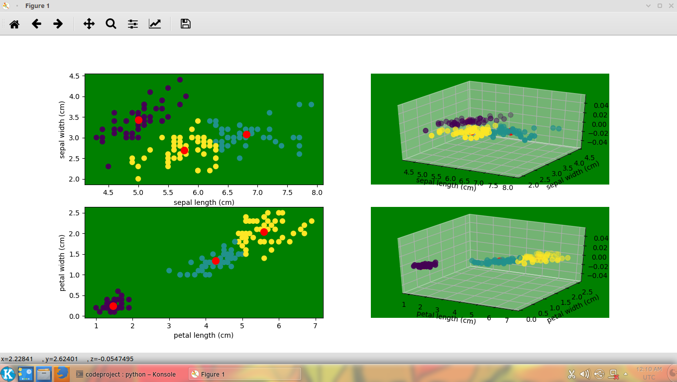
Running the above code shows the following output:

Following is the implementation of the MeanShift clustering.

We create two MeanShift objects and fit the sepal and petal data as follows:

from sklearn.cluster import MeanShift
ms1=MeanShift(n_jobs=-1).fit(sepal_data)
centroids_sepals=ms1.cluster_centers_
labels_sepals=ms1.labels_
ms2=MeanShift(n_jobs=-1).fit(petal_data)
centroids_petals=ms2.cluster_centers_
labels_petals=ms2.labels_

Other steps are same as KMeans clustering. Following is the output of MeanShift clustering:

Note that in MeanShift clustering, the number of clusters is automatically determined by the MeanShift algorithm.

The scipy.cluster.vq module provides the kmeans2 function to implement kmeans clustering. But it requires the data to be normalized before clustering. We can normalize the data by using the whiten function. We can implement kmeans clustering using scipy.cluster.vq module as follows:

# Clustering using KMeans and Scipy

from sklearn import datasets
from scipy.cluster.vq import kmeans2,whiten
import matplotlib.pyplot as plt
from mpl_toolkits.mplot3d import Axes3D

iris=datasets.load_iris()
sepal_data=iris.data[:,0:2]
petal_data=iris.data[:,2:4]
sepal_data_w=whiten(sepal_data)
petal_data_w=whiten(petal_data)
centroids_sepals,labels_sepals=kmeans2(k=3,data=sepal_data_w)
centroids_petals,labels_petals=kmeans2(k=3,data=petal_data_w)
fig=plt.figure()
ax1=fig.add_subplot(221)
ax2=fig.add_subplot(222,projection="3d")
ax3=fig.add_subplot(223)
ax4=fig.add_subplot(224,projection="3d")
ax1.scatter(sepal_data_w[:,0],sepal_data_w[:,1],c=labels_sepals,s=50)
ax1.scatter(centroids_sepals[:,0],centroids_sepals[:,1],c="red",s=100)
ax2.scatter(sepal_data_w[:,0],sepal_data_w[:,1],c=labels_sepals,s=50)
ax2.scatter(centroids_sepals[:,0],centroids_sepals[:,1],c="red",s=100)
ax3.scatter(petal_data_w[:,0],petal_data_w[:,1],c=labels_petals,s=50)
ax3.scatter(centroids_petals[:,0],centroids_petals[:,1],c="red",s=100)
ax4.scatter(petal_data_w[:,0],petal_data_w[:,1],c=labels_petals,s=50)
ax4.scatter(centroids_petals[:,0],centroids_petals[:,1],c="red",s=100)
ax1.set(xlabel=iris.feature_names[0],ylabel=iris.feature_names[1])
ax2.set(xlabel=iris.feature_names[0],ylabel=iris.feature_names[1])
ax3.set(xlabel=iris.feature_names[2],ylabel=iris.feature_names[3])
ax4.set(xlabel=iris.feature_names[2],ylabel=iris.feature_names[3])
ax1.set_facecolor("green")
ax2.set_facecolor("green")
ax3.set_facecolor("green")
ax4.set_facecolor("green")
plt.show()

The above code produces the following output:

Points of Interest

Data clustering is a very useful feature of data mining which finds many practical uses in the field of data classification and image processing. I hope readers find the article useful in understanding the concepts of data clustering.

History

• 28^th October, 2019: Initial version