
Machine Learning Library for C++ (No Dependencies)
5.00/5 (16 votes)
Dependency free machine learning library for C++
Introduction
Although Python has amazing scikit learn library, porting it into native C++ is difficult. Existing machine learning libraries in C++ have too many dependencies. So I have tried my level best to implement some of the most used algorithms in C++. This library is currently in development and I will add many algorithms in future.
My github repository: https://github.com/VISWESWARAN1998/sklearn
Label Encoding
Label encoding is the process of encoding the categorical data into numerical data. For example, if a column in the dataset contains country values like GERMANY, FRANCE, ITALY, then label encoder will convert this categorical data into numerical data like this:
| Country(Categorical) | Country(Numerical) |
GERMANY | 1 |
FRANCE | 0 |
ITALY | 2 |
Here is an example program using our library:
// SWAMI KARUPPASWAMI THUNNAI

#include <iostream>
#include <string>
#include "preprocessing.h"

int main()
{
    std::vector<std::string> categorical_data = { "GERMANY", "FRANCE", "ITALY" };
    LabelEncoder<std::string> encoder(categorical_data);
    std::vector<unsigned long int> numerical_data = encoder.fit_transorm();
    for (int i = 0; i < categorical_data.size(); i++)
    {
        std::cout << categorical_data[i] << " - " << numerical_data[i] << "\n";
    }
}
LabelBinarizer
Label binarize is the most suitable categorical variables like I.P addresses because sometimes while predicting, you may encounter a variable that is not present in the training. LabelEncoder will fail in this case as it has never seen the categorical data before so it cannot convert it into numerical data. But LabelBinarizer works similar to one hot encoder and it will encode all the values to 0 if there is something new while predicting. Below is an example:
// SWAMI KARUPPASWAMI THUNNAI

#include <iostream>
#include <string>
#include "preprocessing.h"

int main()
{
    std::vector<std::string> ip_addresses = { "A", "B", "A", "B", "C" };
    LabelBinarizer<std::string> binarize(ip_addresses);
    std::vector<std::vector<unsigned long int>> result = binarize.fit();
    for (std::vector<unsigned long int> i : result)
    {
        for (unsigned long int j : i) std::cout << j << " ";
        std::cout << "\n";
    }
    // Predict
    std::cout << "Prediction:\n-------------\n";
    std::string test = "D";
    std::vector<unsigned long int> prediction = binarize.predict(test);
    for (unsigned long int i : prediction) std::cout << i << " ";
}
In the above code, we have a feature column of something like this:
A
B
A
B
C
But while predicting, we encounter something entirely new, say "D" from the above example, this is what Label Binarizer will produce.
Output
1 0 0
0 1 0
1 0 0
0 1 0
0 0 1
Prediction:
-------------
0 0 0
Binarizer will find total unique values in training, i.e., A, B, C and will mark each row with 1 where the value is present.
Standardization
StandardScaler will standardize features by removing the mean and scaling to unit variance. Python's scikit learn offers this in the name of "StandardScaler" refer more in their documentation: https://scikit-learn.org/stable/modules/generated/sklearn.preprocessing.StandardScaler.html
Our library offers two methods:
scale: Removes mean and scales to unit varianceinverse_scale: Does the opposite
// SWAMI KARUPPASWAMI THUNNAI

#include <iostream>
#include "preprocessing.h"

int main()
{
    StandardScaler scaler({0, 0, 1, 1});
    std::vector<double> scaled = scaler.scale();
    // Scaled value and inverse scaling
    for (double i : scaled)
    {
        std::cout << i << " " << scaler.inverse_scale(i) << "\n";
    }
}
Normalization
Normalization helps in speeding up the training time.
// SWAMI KARUPPASWAMI THUNNAI

#include <iostream>
#include "preprocessing.h"

int main()
{
    std::vector<double> normalized_vec =
         preprocessing::normalize({ 800, 10, 12, 78, 56, 49, 7, 1200, 1500 });
    for (double i : normalized_vec) std::cout << i << " ";
}
Simple Linear Regression
Simple linear regression consists of only one independent variable X and dependent variable y. We will use https://www.kaggle.com/venjktry/simple-linear-regression/data dataset from kaggle.
Here is an example code which is trained on the above data:
// SWAMI KARUPPASWAMI THUNNAI

#include <iostream>
#include <string>
#include <fstream>
#include "lsr.h"

int main()
{
    simple_linear_regression slr({ 24.0, 50.0, 15.0, 38.0, 87.0, 36.0,
           12.0, 81.0, 25.0, 5.0, 16.0, 16.0, 24.0, 39.0, 54.0, 60.0,
           26.0, 73.0, 29.0, 31.0, 68.0, 87.0, 58.0, 54.0, 84.0, 58.0,
           49.0, 20.0, 90.0, 48.0, 4.0, 25.0, 42.0, 0.0, 60.0, 93.0, 39.0,
           7.0, 21.0, 68.0, 84.0, 0.0, 58.0, 19.0, 36.0, 19.0, 59.0, 51.0,
           19.0, 33.0, 85.0, 44.0, 5.0, 59.0, 14.0, 9.0, 75.0, 69.0, 10.0,
           17.0, 58.0, 74.0, 21.0, 51.0, 19.0, 50.0, 24.0, 0.0, 12.0, 75.0,
           21.0, 64.0, 5.0, 58.0, 32.0, 41.0, 7.0, 4.0, 5.0, 49.0, 90.0, 3.0,
           11.0, 32.0, 83.0, 25.0, 83.0, 26.0, 76.0, 95.0, 53.0, 77.0, 42.0,
           25.0, 54.0, 55.0, 0.0, 73.0, 35.0, 86.0, 90.0, 13.0, 46.0, 46.0,
           32.0, 8.0, 71.0, 28.0, 24.0, 56.0, 49.0, 79.0, 90.0, 89.0, 41.0,
           27.0, 58.0, 26.0, 31.0, 70.0, 71.0, 39.0, 7.0, 48.0, 56.0, 45.0,
           41.0, 3.0, 37.0, 24.0, 68.0, 47.0, 27.0, 68.0, 74.0, 95.0, 79.0,
           21.0, 95.0, 54.0, 56.0, 80.0, 26.0, 25.0, 8.0, 95.0, 94.0, 54.0,
           7.0, 99.0, 36.0, 48.0, 65.0, 42.0, 93.0, 86.0, 26.0, 51.0, 100.0,
           94.0, 6.0, 24.0, 75.0, 7.0, 53.0, 73.0, 16.0, 80.0, 77.0, 89.0, 80.0,
           55.0, 19.0, 56.0, 47.0, 56.0, 2.0, 82.0, 57.0, 44.0, 26.0, 52.0, 41.0,
           44.0, 3.0, 31.0, 97.0, 21.0, 17.0, 7.0, 61.0, 10.0, 52.0, 10.0, 65.0,
           71.0, 4.0, 24.0, 26.0, 51.0 }, { 21.54945196, 47.46446305, 17.21865634,
           36.58639803, 87.28898389, 32.46387493, 10.78089683, 80.7633986, 24.61215147,
           6.963319071, 11.23757338, 13.53290206, 24.60323899, 39.40049976, 48.43753838,
           61.69900319, 26.92832418, 70.4052055, 29.34092408, 25.30895192, 69.02934339,
           84.99484703, 57.04310305, 50.5921991, 83.02772202, 57.05752706, 47.95883341,
           24.34226432, 94.68488281, 48.03970696, 7.08132338, 21.99239907, 42.33151664,
           0.329089443, 61.92303698, 91.17716423, 39.45358014, 5.996069607, 22.59015942,
           61.18044414, 85.02778957, -1.28631089, 61.94273962, 21.96033347, 33.66194193,
           17.60946242, 58.5630564, 52.82390762, 22.1363481, 35.07467353, 86.18822311,
           42.63227697, 4.09817744, 61.2229864, 17.70677576, 11.85312574, 80.23051695,
           62.64931741, 9.616859804, 20.02797699, 61.7510743, 71.61010303, 23.77154623,
           51.90142035, 22.66073682, 50.02897927, 26.68794368, 0.376911899, 6.806419002,
           77.33986001, 28.90260209, 66.7346608, 0.707510638, 57.07748383, 28.41453196,
           44.46272123, 7.459605998, 2.316708112, 4.928546187, 52.50336074, 91.19109623,
           8.489164326, 6.963371967, 31.97989959, 81.4281205, 22.62365422, 78.52505087,
           25.80714057, 73.51081775, 91.775467, 49.21863516, 80.50445387, 50.05636123,
           25.46292549, 55.32164264, 59.1244888, 1.100686692, 71.98020786, 30.13666408,
           83.88427405, 89.91004752, 8.335654576, 47.88388961, 45.00397413, 31.15664574,
           9.190375682, 74.83135003, 30.23177607, 24.21914027, 57.87219151, 50.61728392,
           78.67470043, 86.236707, 89.10409255, 43.26595082, 26.68273277, 59.46383041,
           28.90055826, 31.300416, 71.1433266, 68.4739206, 39.98238856, 4.075776144,
           47.85817542, 51.20390217, 43.9367213, 38.13626679, 3.574661632, 36.4139958,
           22.21908523, 63.5312572, 49.86702787, 21.53140009, 64.05710234, 70.77549842,
           92.15749762, 81.22259156, 25.10114067, 94.08853397, 53.25166165, 59.16236621,
           75.24148428, 28.22325833, 25.33323728, 6.364615703, 95.4609216, 88.64183756,
           58.70318693, 6.815491279, 99.40394676, 32.77049249, 47.0586788, 60.53321778,
           40.30929858, 89.42222685, 86.82132066, 26.11697543, 53.26657596, 96.62327888,
           95.78441027, 6.047286687, 24.47387908, 75.96844763, 3.829381009, 52.51703683,
           72.80457527, 14.10999096, 80.86087062, 77.01988215, 86.26972444, 77.13735466,
           51.47649476, 17.34557531, 57.72853572, 44.15029394, 59.24362743, -1.053275611,
           86.79002254, 60.14031858, 44.04222058, 24.5227488, 52.95305521, 43.16133498,
           45.67562576, -2.830749501, 29.19693178, 96.49812401, 22.5453232, 20.10741433,
           4.035430253, 61.14568518, 13.97163653, 55.34529893, 12.18441166, 64.00077658,
           70.3188322, -0.936895047, 18.91422276, 23.87590331, 47.5775361 }, DEBUG);
    slr.fit();
    std::vector<double> test = { 45.0, 91.0, 61.0, 10.0, 47.0, 33.0, 84.0, 24.0, 48.0,
    48.0, 9.0, 93.0, 99.0, 8.0, 20.0, 38.0, 78.0, 81.0, 42.0, 95.0, 78.0, 44.0, 68.0, 87.0,
    58.0, 52.0, 26.0, 75.0, 48.0, 71.0, 77.0, 34.0, 24.0, 70.0, 29.0, 76.0, 98.0, 28.0, 87.0,
    9.0, 87.0, 33.0, 64.0, 17.0, 49.0, 95.0, 75.0, 89.0, 81.0, 25.0, 47.0, 50.0, 5.0, 68.0,
    84.0, 8.0, 41.0, 26.0, 89.0, 78.0, 34.0, 92.0, 27.0, 12.0, 2.0, 22.0, 0.0, 26.0, 50.0,
    84.0, 70.0, 66.0, 42.0, 19.0, 94.0, 71.0, 19.0, 16.0, 49.0, 29.0, 29.0, 86.0, 50.0,
    86.0, 30.0, 23.0, 20.0, 16.0, 57.0, 8.0, 8.0, 62.0, 55.0, 30.0, 86.0, 62.0,
    51.0, 61.0, 86.0, 61.0, 21.0 };
    for (double i : test)
    {
        std::ofstream file;
        file.open("out.txt", std::ios::app);
        file << slr.predict(i);
        file << "\n";
        file.close();
    }
    slr.save_model("model.sklearn");
    int stay;
    std::cin >> stay;
}
We have visualized our C++ model's prediction:

class: simple_linear_regression
Constructor for Training a New Model
// independent variable X, dependent variable y, DEBUG/NODEBUG will print verbose messages
simple_linear_regression(std::vector<double> X, std::vector<double> y, unsigned short verbose);
We then use the fit method to train the model.
Constructor for Loading the Saved Model
simple_linear_regression(std::string model_name);
Multiple Linear Regression
Simple linear regression has only one independent variable whereas multiple linear regression has many two or more independent variables. Solving this involves matrix algebra and it consumes some adequate time if you have many independent variables and a bigger dataset.
Here is an example dataset on predicting the test score from IQ and study hours from stattrek:

Training and Saving the Model
// SWAMI KARUPPASWAMI THUNNAI

#include <iostream>
#include "mlr.h"

int main()
{
    LinearRegression mlr({ {110, 40}, {120, 30}, {100, 20}, {90, 0},
                         {80, 10} }, {100, 90, 80, 70, 60}, NODEBUG);
    mlr.fit();
    std::cout << mlr.predict({ 110, 40 });
    mlr.save_model("model.json");
}
Loading the Saved Model
// SWAMI KARUPPASWAMI THUNNAI

#include <iostream>
#include "mlr.h"

int main()
{
    // Don't use fit method here
    LinearRegression mlr("model.json");
    std::cout << mlr.predict({ 110, 40 });
}
Logistic Regression
Please do not get confused with the word "regression" in Logistic regression. It is generally used for classification problems. The heart of the logistic regession is sigmoid activation function. An activation function is a function which takes any input value and outputs value within a certain case. In our case(sigmoid), it returns between 0 and 1.
In the image, you can see the output(y) of sigmoid activation function for -3 >= x <= 3

The idea behind the logistic regression is taking the output from linear regression, i.e., y = mx+c and applying logistic function 1/(1+e^-y) which outputs the value between 0 and 1. We can clearly see this is a binary classifier, i.e., for example, it can be used for classifying binary datasets like predicting whether it is a male or a female using certain parameters.
But we can use this logistic regression to classify multi-class problems too with some modifications. Here, we are using the one vs rest principle. That is training many linear regression models, for example, if the class count is 10, it will train 10 Linear Regression models by changing the class values with 1 as the class value to predict the probability and 0 to the rest. If you don't understand, here is a detailed explanation: https://prakhartechviz.blogspot.com/2019/02/multi-label-classification-python.html
We are going to take a simple classification problem to classify whether it is a male or female.
Classification male - female using height, weight, foot size and saving the model. Here is our dataset:

All we have to do is to predict whether the person is male or female using height, weight and foot size.
// SWAMI KARUPPASWAMI THUNNAI

#include <iostream>
#include "logistic_regression.h"

int main()
{
    logistic_regression lg({ { 6, 180, 12 },{ 5.92, 190, 11 },{ 5.58, 170, 12 },
        { 5.92, 165, 10 },{ 5, 100, 6 },{ 5.5, 150, 8 },{ 5.42, 130, 7 },{ 5.75, 150, 9 } },
        { 0, 0, 0, 0, 1, 1, 1, 1 }, NODEBUG);
    lg.fit();
    // Save the model
    lg.save_model("model.json");
    std::map<unsigned long int, double> probabilities = lg.predict({ 6, 130, 8 });
    double male = probabilities[0];
    double female = probabilities[1];
    if (male > female) std::cout << "MALE";
    else std::cout << "FEMALE";
}
and loading a saved model:
// SWAMI KARUPPASWAMI THUNNAI

#include <iostream>
#include "logistic_regression.h"

int main()
{
    logistic_regression lg("model.json");
    std::map<unsigned long int, double> probabilities = lg.predict({ 6, 130, 8 });
    double male = probabilities[0];
    double female = probabilities[1];
    if (male > female) std::cout << "MALE";
    else std::cout << "FEMALE";
}
Gaussian Naive Bayes
Classification male - female using height, weight, foot size and saving the model. Here is our dataset:
Training a Model
// SWAMI KARUPPASWAMI THUNNAI

#include "naive_bayes.h"

int main()
{
    gaussian_naive_bayes nb({ {6, 180, 12}, {5.92, 190, 11}, {5.58, 170, 12},
    {5.92, 165, 10}, {5, 100, 6}, {5.5, 150, 8}, {5.42, 130, 7}, {5.75, 150, 9} },
    { 0, 0, 0, 0, 1, 1, 1, 1 }, DEBUG);
    nb.fit();
    nb.save_model("model.json");
    std::map<unsigned long int, double> probabilities = nb.predict({ 6, 130, 8 });
    double male = probabilities[0];
    double female = probabilities[1];
    if (male > female) std::cout << "MALE";
    else std::cout << "FEMALE";
}
Loading a Saved Model
// SWAMI KARUPPASWAMI THUNNAI

#include "naive_bayes.h"

int main()
{
    gaussian_naive_bayes nb(NODEBUG);
    nb.load_model("model.json");
    std::map<unsigned long int, double> probabilities = nb.predict({ 6, 130, 8 });
    double male = probabilities[0];
    double female = probabilities[1];
    if (male > female) std::cout << "MALE";
    else std::cout << "FEMALE";
}
Training Bigger Datasets
Usually, machine learning datasets are huge even simple alogrithms perform well when enough data is provided[8]. We cannot write the dataset as vectors in the source code itself, we need some way to take the dataset from the data dynamically. Here, we will convert the dataset into JSON format using your favorite programming language like this.
You can see the dataset here: https://github.com/VISWESWARAN1998/sklearn/blob/master/datasets/boston_house_prices.json

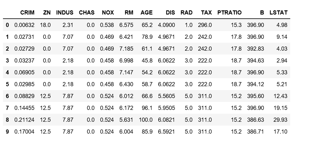
where max_index is total rows present and every row has X and y which is independent and dependent variables. Once trained, we can use noob_pandas class which is shipped with this library to get the independent and dependent variables. Here, I will show you how to train famous Boston Housing dataset.
https://medium.com/@yharsh800/boston-housing-linear-regression-robust-regression-9be52132def4
The labels present in the dataset:

and a few values of how our data looks like:
Training and Predicting Using Boston Dataset
// SWAMI KARUPPASWAMI THUNNAI

#include <iostream>
#include "mlr.h"
#include "noob_pandas.h"

int main()
{
    // For classification use unsigned long int instead of double
    noob_pandas<double> dataset("boston_house_prices.json");
    LinearRegression mlr(dataset.get_X(), dataset.get_y(), NODEBUG);
    mlr.fit();
    std::cout << mlr.predict({ 0.02729, 0.0, 7.07, 0.0, 0.469,
                               7.185, 61.1, 4.9671, 2.0, 242.0, 17.8, 392.83, 4.03 });
}
*Note: I will post how I made the json dataset in the comment below, I have used Python programming language and I am sure you can use other language you wish.
References
- https://scikit-learn.org/stable/
- https://hackernoon.com/implementation-of-gaussian-naive-bayes-in-python-from-scratch-c4ea64e3944d
- https://www.mathsisfun.com/data/least-squares-regression.html
- https://www.antoniomallia.it/lets-implement-a-gaussian-naive-bayes-classifier-in-python.html
- https://www.geeksforgeeks.org/adjoint-inverse-matrix/
- https://stattrek.com/multiple-regression/regression-coefficients.aspx
- https://en.wikipedia.org/wiki/Sigmoid_function
- http://static.googleusercontent.com/media/research.google.com/fr//pubs/archive/35179.pdf
History
- 2019-09-22: Initial release
- 2019-09-30: New algorithm, bug fixes
- 2019-10-08 New algorithms, bug fixes, optimization and refactoring