An Introduction to Support Vector Machine (SVM) and the Simplified SMO Algorithm

Introduction

In machine learning, support vector machines (SVMs) are supervised learning models with associated learning algorithms that analyze data used for classification and regression analysis (Wikipedia). This article is a summary of my learning and the main sources can be found in the References section.

Support Vector Machines and the Sequential Minimal Optimization (SMO) can be found in [1],[2] and [3]. Details about a simplified version of the SMO and its pseudo-code can be found in [4]. You can also find Python code of the SMO algorithms in [5] but it is hard to understand for beginners who have just started to learn Machine Learning. [6] is a special gift for beginners who want to learn about Support Vector Machine basically. In this article, I am going to introduce about SVM and a simplified version of the SMO by using Python code based on [4].

Background

In this article, we will consider a linear classifier for a binary classification problem with labels y (y ϵ [-1,1]) and features x. A SVM will compute a linear classifier (or a line) of the form:

With f(x), we can predict y = 1 if f(x) ≥ 0 and y = -1 if f(x) < 0. And by solving the dual problem (Equation 12, 13 in [1] at the References section), f(x) can be expressed:

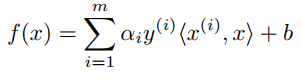
where α_i (alpha i) is a Lagrange multiplier for solution and <x(ⁱ⁾,x> called inner product of x⁽ⁱ⁾ and x. A Python version of f(x) maybe look like this:

fXi = float(multiply(alphas,Y).T*(X*X[i,:].T)) + b

The Simplified SMO Algorithm

The simplified SMO algorithm takes two α parameters, α_i and α_j, and optimizes them. To do this, we iterate over all α_i, i = 1, . . . m. If α_i does not fulfill the Karush-Kuhn-Tucker conditions to within some numerical tolerance, we select α_j at random from the remaining m − 1 α’s and optimize α_i and α_j. The following function is going to help us to select j randomly:

def selectJrandomly(i,m):
      j=i
      while (j==i):
            j = int(random.uniform(0,m))
      return j

If none of the α’s are changed after a few iterations over all the α_i’s, then the algorithm terminates. We must also find bounds L and H:

• If y⁽ⁱ⁾ != y^(j), L = max(0, α_j − α_i), H = min(C, C + α_j − α_i)
• If y⁽ⁱ⁾ = y^(j), L = max(0, α_i + α_j − C), H = min(C, α_i + α_j)

Where C is a regularization parameter. Python code for the above is as follows:

if (Y[i] != Y[j]):
      L = max(0, alphas[j] - alphas[i])
      H = min(C, C + alphas[j] - alphas[i])
else:
      L = max(0, alphas[j] + alphas[i] - C)
      H = min(C, alphas[j] + alphas[i])

Now, we are going to find α_j is given by:

Python code:

alphas[j] -= Y[j]*(Ei - Ej)/eta

Where:

Python code:

Ek = fXk - float(Y[k])
eta = 2.0 * X[i,:]*X[j,:].T - X[i,:]*X[i,:].T - X[j,:]*X[j,:].T

If this value ends up lying outside the bounds L and H, we must clip the value of α_j to lie within this range:

The following function is going to help us to clip the value α_j:

def clipAlphaJ(aj,H,L):
      if aj > H:
            aj = H
      if L > aj:
            aj = L
      return aj

Finally, we can find the value for α_i. This is given by:

where α^(old)_j is the value of α_j before optimization. A version of Python code can look like this:

alphas[i] += Y[j]*Y[i]*(alphaJold - alphas[j])

After optimizing α_i and α_j, we select the threshold b:

where b₁:

and b₂:

Python code for b₁ and b₂:

b1 = b - Ei- Y[i]*(alphas[i]-alphaIold)*X[i,:]*X[i,:].T - Y[j]*(alphas[j]-alphaJold)*X[i,:]*X[j,:].T
b2 = b - Ej- Y[i]*(alphas[i]-alphaIold)*X[i,:]*X[j,:].T - Y[j]*(alphas[j]-alphaJold)*X[j,:]*X[j,:].T

Computing the W

After optimizing α_i and α_j, we can also compute w that is given:

The following function helps us to compute w from α_i and α_j:

def computeW(alphas, dataX, classY):
      X = mat(dataX)
      Y = mat(classY).T
      m,n = shape(X)
      w = zeros((n,1))
      for i in range(m):
            w += multiply(alphas[i]*Y[i],X[i,:].T)
      return w

Predicted Class

We can predict which class a point belongs to from w and b:

def predictedClass(point, w, b):
      p = mat(point)
      f = p*w + b
      if f > 0:
            print(point," is belong to Class 1")
      else:
            print(point," is belong to Class -1")

The Python Function for the Simplified SMO Algorithm

And now, we can create a function (named simplifiedSMO) for the simplified SMO algorithm based on pseudo code in [4]:

Input

• C: regularization parameter
• tol: numerical tolerance
• max passes: max # of times to iterate over α’s without changing
• (x⁽¹⁾, y⁽¹⁾), . . . , (x^(m), y^(m)): training data

Output

α : Lagrange multipliers for solution

b : threshold for solution

def simplifiedSMO(dataX, classY, C, tol, max_passes):
       X = mat(dataX);
       Y = mat(classY).T
       m,n = shape(X)
       # Initialize b: threshold for solution
       b = 0;      
       # Initialize alphas: lagrange multipliers for solution
       alphas = mat(zeros((m,1)))
       passes = 0
       while (passes < max_passes):
              num_changed_alphas = 0
              for i in range(m):
                     # Calculate Ei = f(xi) - yi
                     fXi = float(multiply(alphas,Y).T*(X*X[i,:].T)) + b
                     Ei = fXi - float(Y[i])
                     if ((Y[i]*Ei < -tol) and (alphas[i] < C)) or ((Y[i]*Ei > tol) 
                                  and (alphas[i] > 0)):
                           # select j # i randomly
                           j = selectJrandom(i,m)
                           # Calculate Ej = f(xj) - yj
                           fXj = float(multiply(alphas,Y).T*(X*X[j,:].T)) + b
                           Ej = fXj - float(Y[j])
                           # save old alphas's
                           alphaIold = alphas[i].copy();
                           alphaJold = alphas[j].copy();
                           # compute L and H
                           if (Y[i] != Y[j]):
                                  L = max(0, alphas[j] - alphas[i])
                                  H = min(C, C + alphas[j] - alphas[i])
                           else:
                                  L = max(0, alphas[j] + alphas[i] - C)
                                  H = min(C, alphas[j] + alphas[i])
                           # if L = H the continue to next i
                           if L==H:
                                  continue
                           # compute eta
                           eta = 2.0 * X[i,:]*X[j,:].T - X[i,:]*X[i,:].T - X[j,:]*X[j,:].T
                           # if eta >= 0 then continue to next i
                           if eta >= 0:
                                  continue
                           # compute new value for alphas j
                           alphas[j] -= Y[j]*(Ei - Ej)/eta
                           # clip new value for alphas j
                           alphas[j] = clipAlphasJ(alphas[j],H,L)
                           # if |alphasj - alphasold| < 0.00001 then continue to next i
                           if (abs(alphas[j] - alphaJold) < 0.00001):
                                  continue
                           # determine value for alphas i
                           alphas[i] += Y[j]*Y[i]*(alphaJold - alphas[j])
                           # compute b1 and b2
                           b1 = b - Ei- Y[i]*(alphas[i]-alphaIold)*X[i,:]*X[i,:].T - 
                                      Y[j]*(alphas[j]-alphaJold)*X[i,:]*X[j,:].T
                           b2 = b - Ej- Y[i]*(alphas[i]-alphaIold)*X[i,:]*X[j,:].T 
                                    - Y[j]*(alphas[j]-alphaJold)*X[j,:]*X[j,:].T
                           # compute b
                           if (0 < alphas[i]) and (C > alphas[i]):
                                  b = b1
                           elif (0 < alphas[j]) and (C > alphas[j]):
                                  b = b2
                           else:
                                  b = (b1 + b2)/2.0                      
                           num_changed_alphas += 1
                     if (num_changed_alphas == 0): passes += 1
                     else: passes = 0
       return b,alphas

Plotting the Linear Classifier

After having alpha, w and b, we can also plot the linear classifier (or a line). The following function is going to help us to do this:

def plotLinearClassifier(point, w, alphas, b, dataX, labelY):
      
       shape(alphas[alphas>0])
      
       Y = np.array(labelY)
       X = np.array(dataX)
       svmMat = []
       alphaMat = []
       for i in range(10):
              alphaMat.append(alphas[i])
              if alphas[i]>0.0:
                     svmMat.append(X[i])
                                 
       svmPoints = np.array(svmMat)
       alphasArr = np.array(alphaMat)

       numofSVMs = shape(svmPoints)[0]
       print("Number of SVM points: %d" % numofSVMs)
 
       xSVM = []; ySVM = []
       for i in range(numofSVMs):
              xSVM.append(svmPoints[i,0])
              ySVM.append(svmPoints[i,1])    
     
       n = shape(X)[0]    
       xcord1 = []; ycord1 = []
       xcord2 = []; ycord2 = []
      
       for i in range(n):
              if int(labelY[i])== 1:
                     xcord1.append(X[i,0])
                     ycord1.append(X[i,1])                  
              else:
                     xcord2.append(X[i,0])
                     ycord2.append(X[i,1])                  

       fig = plt.figure()
       ax = fig.add_subplot(111)
       ax.scatter(xcord1, ycord1, s=30, c='red', marker='s')
       for j in range(0,len(xcord1)):
              for l in range(numofSVMs):
                     if (xcord1[j]== xSVM[l]) and (ycord1[j]== ySVM[l]):
                           ax.annotate("SVM", (xcord1[j],ycord1[j]), (xcord1[j]+1,ycord1[j]+2),
                                      arrowprops=dict(facecolor='black', shrink=0.005))
      
       ax.scatter(xcord2, ycord2, s=30, c='green')
       for k in range(0,len(xcord2)):
              for l in range(numofSVMs):
                     if (xcord2[k]== xSVM[l]) and (ycord2[k]== ySVM[l]):
                           ax.annotate("SVM", (xcord2[k],ycord2[k]),(xcord2[k]-1,ycord2[k]+1),
                                 arrowprops=dict(facecolor='black', shrink=0.005))
      
       red_patch = mpatches.Patch(color='red', label='Class 1')
       green_patch = mpatches.Patch(color='green', label='Class -1')
       plt.legend(handles=[red_patch,green_patch])
      
       x = []
       y = []
       for xfit in np.linspace(-3.0, 3.0):
              x.append(xfit)
              y.append(float((-w[0]/w[1])*xfit - b[0,0])/w[1])
             
       ax.plot(x,y)
      
       predictedClass(point,w,b)
       p = mat(point)
       ax.scatter(p[0,0], p[0,1], s=30, c='black', marker='s')
       circle1=plt.Circle((p[0,0],p[0,1]),0.6, color='b', fill=False)
       plt.gcf().gca().add_artist(circle1)
      
       plt.show()

Using the Code

To run all of Python code above, we need to create three files:

• The myData.txt file contains training data:

  -3 -2 0
  -2 3 0
  -1 -4 0
  2 3 0
  3 4 0
  -1 9 1
  2 14 1
  1 17 1
  3 12 1
  0 8 1

  In each row, the two first values are features and the third value is a label.

• The SimSMO.py file contains functions:
  Python

  def loadDataSet(fileName):
         dataX = []
         labelY = []
         fr = open(fileName)
         for r in fr.readlines():
                record = r.strip().split()
                dataX.append([float(record[0]), float(record[1])])
                labelY.append(float(record[2]))
         return dataX, labelY
  # select j # i randomly
  def selectJrandomly(i,m):
  ...
  # clip new value for alphas j
  def clipAlphaJ(alphasj,H,L):
  ...
  def simplifiedSMO(dataX, classY, C, tol, max_passes):
  ...
  def computeW(alphas,dataX,classY):
  ...
  def plotLinearClassifier(point, w, alphas, b, dataX, labelY):
  ...
  def predictedClass(point, w, b):
  ...

• Finally, we need to create the testSVM.py file to test functions:
  Python

  import SimSMO
  X,Y = SimSMO.loadDataSet('myData.txt')
  b,alphas = SimSMO.simplifiedSMO(X, Y, 0.6, 0.001, 40)
  w = SimSMO.computeW(alphas,X,Y)
  # test with the data point (3, 4)
  SimSMO.plotLinearClassifier([3,4], w, alphas, b, X, Y)

The result can look like this:

Number of SVM points: 3
[3, 4]  is belong to Class -1

And:

Points of Interest

In this article, I only introduced the SVM basically and a simplified version of the SMO algorithm. If you want to use SVMs and the SMO in a real world application, you can discover more about them in documents below (or maybe more).

References

• [1] CS229 Lecture notes, Andrew Ng, Support Vector Machines
• [2] Bingyu Wang, Virgil Pavlu, Support Vector Machines
• [3] John C. Platt, Fast Training of Support Vector Machines using Sequential Minimal Optimization
• [4] CS 229, Autumn 2009, The simplified SMO Algorithm
• [5] Peter Harrington, Machine learning in Action
• [6] Alexandre Kowalczyk, Support Vector Machines Succinctly

History

• 18^th November, 2018: Initial version