
Ability of the L-system in R Comparing to Well-known Tools
5.00/5 (2 votes)
Demonstrating ability of the L-system in R, and offering helper functions able to plot all main categories of figures typical for the 2D L-system.
Introduction
Lindenmayer system (or L-system) [1,2] is a powerful tool to generate amazing figures, especially curves, trees, plants, etc. Usually, it is using such input parameters as order, angles, axiom, production rules, etc. Based on all of them L-system is generating figures.
LindenmayeR package in R (LPR) [3] supports 2D L-system, but only basic features, even if compare them to described in the old classic book [1]. It was proved by author of this article that the LPR can produce a majority of samples that could be found in books, papers or on Internet. Not to mention, - adding color in many cases makes figures look more attractive and meaningful.
There are a few very good online generators based on L-system common rules [4,5]. They could be used (and were used) for additional testing of any new figures, also to compare different results, including the LPR results. But take into account, that some generators are using different or advanced features if compare them to the LPR. It means that in some cases it's impossible to use some found samples "as is", they require sort of "translation" to the LPR rules, and in some cases even a translation is not working.
It should be mentioned, that it is hard to find the new interesting samples online (excluding [1-5]). In other cases, it is possible to fix shown unique figures. E.g., I've found Sierpinski carpet in [4], and spent some time to dissect it and fix it (i.e., delete extra lines). It means that the LPR is a little bit more flexible than some other tools. So, compare the LPR results to some fractals produced using different tools, e.g., found in [6,7].
Creating curves and using helper function and template
To complete such an intense testing and a comparison in a timely manner, - the set of a helper function and a helper function-template were created for the LPR.
Note: the functions created using a template are sort of helper functions too.
The prime goal of this set is to make using of the package functionality very clear, understandable and easy.
A good helper function, usually, encapsulates typical set of actions for current tasks, supplies often used default values, interacting with other helper functions, etc. Presented here functions help a user to avoid complexity of the package functionality and concentrate on prime arguments used in function calls. It is especially useful during an initial testing of the new figure. Also, even more important during preparing a presentation, when mass testing and retesting occurs , e.g., applying different orders and sizes, colors, etc.
In such cases, helper functions assisted to make process of testing hundreds of samples a little bit "automated". E.g., if file name and/or title are empty strings then they wold be generated from short name. It will save user time for sure. So, usually (and mostly) user now need only to set 6 arguments (after defining prime rules for initial testing), i.e.:
- The abbreviated name of a figure (which would be used for an output log and for generating the plotted file name);
- The order and a distance unit (defining a size and a placement of the figure);
- Starting x,y coordinates and the color.
Later, only a unit distance and starting x,y coordinates are used to place a figure nicely on a canvas.
There are only 1 plotting helper function pLPRF() and 1 plotting helper function-template pXXXX() for building any particular figure. Because the pLPRF() function almost always is unmodified, only building any pXXXX() would be described by examples.
It's recommended to build pXXXX() in a few simple steps:
- First of all, set such important parameters as fign - a figure short, abbreviated name (used for an output log, also to build a plot file name, etc.) and ttl - a title.
- Next, set all prime parameters defining selected to create figure. They are following: an order, a regular angle, an axiom and production rules represented with 2 lists, i.e., inpr=c(...); outr=c(...);.
- Last, set any additional parameters that could be stable, unchanged. E.g., an initial angle, chars, or even a color.
OK, now let's create the prime function generating and plotting the "Row of trees, A" figure.
In downloaded zip-file find the ILPR_A4_hft.txt with the following template (a little bit simplified here):
## <<Type any description here>>
#pXXXX <- function(ord, du, x=2, y=2, clr) {
#  fign="XXXX"; ttl="YYYYY";
#  axiom="U...";
#  inpr=c("A,..."); outr=c("B,...");
#  symc=c("F",...,"+","-","[","]"); actc=symc;  ## or add actc=<<needed chars>>
#  ar=90; ai=0; strt=c(x,y,ai);
#  #cat(" *** pars:",ord,du,strt,ttl,"\n",axiom,"/", inpr,"/", outr,"\n",
   #symc,"/", actc,"\n"); ## 4 testing
#  pLPRF(ord, du, strt, ar, clr, fign,, ttl, axiom, inpr, outr, symc, actc)
#}
#pXXXX(3,1,2,2,"red")
Here are definitions of arguments pulled from pLPRF() to remind us what is what.
## Where: ord - order/level; du - distance unit; strt - starting values:
## c(x,y,ai), where ai is an init angle; ar - regular angle; clr - color;
## fign - figure short name; fn - file name; ttl - plot title; inpr - input
## rules; outr - output rules; symc - symbol chars; actc - action chars.
Now we will replace "placeholders" like "XXXX", "YYYY" and others with real values we need.
The first and last 3 lines are looking now like this:
## Plotting "Row of trees, A" curve [ar=86], a.k.a. Cesaro curve
pROTA <- function(ord, du, x=2, y=2, clr) {
  fign="ROTA"; ttl="Row of trees, A";
## <<still need to add here an axiom, rules, etc.>>
  pLPRF(ord, du, strt, ar, clr, fign,, ttl, axiom, inpr, outr, symc, actc)  ## keep unchanged
}
pROTA(6,1,2,2,"red")
After going on with 2 final steps we have the required function:
## Plotting "Row of trees, A" curve [ar=86], a.k.a. Cesaro curve
pROTA <- function(ord, du, x=2, y=2, clr) {
  fign="ROTA"; ttl="Row of trees, A";
  axiom="F";
  inpr=c("F"); outr=c("F+F--F+F");
  symc=c("F","+","-","[","]"); actc=symc;
  ar=86; ai=0; strt=c(x,y,ai);
  pLPRF(ord, du, strt, ar, clr, fign,, ttl, axiom, inpr, outr, symc, actc)
}
pROTA(6,1,2,2,"darkgreen")
It is recommended to use this template style for all functions you will create. For this paper a more compact style is used usually.
Here is another additional introductory sample of the already created function:
## Plotting Penrose tiling
pPRT <- function(ord, du, x=2, y=2, clr) {
  fign="PRT"; ttl="Penrose tiling"; ar=36; ai=0; strt=c(x,y,ai);
  axiom="[7]++[7]++[7]++[7]++[7]";
  inpr=c("7","6","8","9"); outr=c("+81--91[---61--71]+",
    "81++91----71[-81----61]++","-61++71[+++81++91]-",
    "--81++++61[+91++++71]--71");
  symc=c("7","6", "8", "9", "+", "-", "[", "]");
  actc = c("F","F","F","F","+","-", "[", "]");
  pLPRF(ord, du, strt, ar, clr, fign,, ttl, axiom, inpr, outr, symc, actc) }
pPRT(5,4,49,49,"navy")
Both introductory samples are presented below in the Fig. 1 and Fig. 2.


Creating and showing the most important categories of figures and curves
Traditionally, the most important categories are following: plants, tries, space filling curves, carpets, rugs, tiles, etc. In each category very familiar, well-known figures will be created and shown, but, at the same time, a few unique figures would be demonstrated too.
From now on find all functions in the ILPR_A4_samples.txt and many additional pictures in the ILPRpsamples.pdf.
Category: Plants
Four selected figures of plants are presented below in Fig. 3 - Fig. 6.


Category: Space filling curves
Four popular types of space filling curves are presented below in Fig. 7 - Fig. 10.


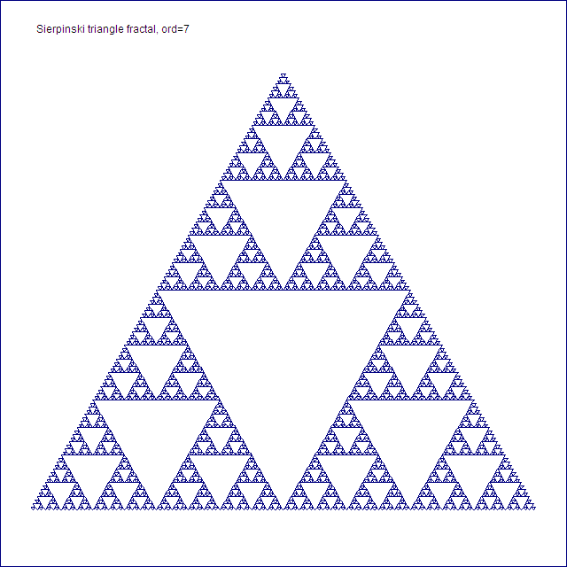
Category: Famous Sierpinski and Koch fractals
All four famous fractals are presented below in Fig. 11 - Fig. 14.


Category: Rugs
Figures called Rugs here have nothing to do with Sierpinski carpet and triangle. They are new type of figures.
Remark: These figures are really looking like small area rugs. Aren't they?
Selected four rugs are presented below in Fig. 15 - Fig. 18.


Category: Dragon and other curves
Selected four curves are presented below in Fig. 19 - Fig. 22.


Find many additional curves in the file ILPRpsamples.pdf.
Conclusion
Presented helper functions for the LPR and plotted images they produced confirmed the great flexibility of the LindenmayeR package, which is able to plot images in all prime categories of the traditional 2D L-system. It should be stressed, that quality of plotted figures is even better than some samples created using other approaches. For example, it is very obvious in the case of the Sierpinski triangle realized in 42 languages on Rosettacode Wiki [8].
The following questions is still opened: Why some very popular fractals (e.g., Sierpinski triangle and carpet) can be plotted using many different algorithms, languages and tools?
In the file ILPR_A4_samples.txt many additional testing samples are provided for all categories of curves to keep you busy and enjoying new curves.
References
- Prusinkiewicz P., Lindenmayer A. (1990), The Algorithmic Beauty of Plants (The Virtual Laboratory), Springer-Verlag, ISBN 0387972978, URL: http://algorithmicbotany.org/papers/abop/abop.pdf.
- L-system, Wikipedia, the free encyclopedia, URL: https://en.wikipedia.org/wiki/L-system.
- Hanson B., LindenmayeR: Functions to Explore L-Systems, URL: https://CRAN.R-project.org/package=LindenmayeR.
- Roast K., L-Systems Turtle Graphics Renderer, URL: http://www.kevs3d.co.uk/dev/lsystems/.
- Noland C. Lindenmayer System Generator, URL:http://nolandc.com/sandbox/fractals/.
- Voevudko, A.E. (2017), Generating Kronecker Product Based Fractals, Code Project, URL: https://www.codeproject.com/Articles/1189288/Generating-Kronecker-Product-Based-Fractals
- Voevudko, A.E. (2017), A Few Approaches to Generating Fractal Images in R, Code Project, URL: https://www.codeproject.com/Articles/1195034/A-Few-Approaches-to-Generating-Fractal-Images-in-R.
- Sierpinski triangle, Rosetta Code Wiki, URL: http://rosettacode.org/wiki/Sierpinski_triangle/Graphical.