Our objective in this article is to determine the superiority of one algorithm over another when faced with two or more options. While we strive for simplicity, there may be instances where we delve into the intricate details as necessary.
Introduction
Everyone appreciates computers for their ability to swiftly accomplish tasks. There is a universal expectation that computers exhibit responsiveness and high performance. However, behind every task assigned to a computer lies a sequence of instructions that must be executed in a specific order. Within this framework, variations can arise in the way instructions are defined, necessitating the exploration of methods that are more efficient than others. The question then arises: how can one determine that one method is superior to another?
Three authoritative textbooks on this topic merit consultation. They are widely recognized as standard references and are universally employed in courses.
So, how can one determine that one method is superior to another?
In reality, there isn't a single definitive answer to this question, as the term "superior" can carry different meanings for each individual. Some may argue that a method is superior if it requires less space in memory, particularly important for devices where memory management is critical, such as microcontrollers. Others may consider a method superior if it is easy to understand and explain. In this series, we will define a method as superior if it simply takes less time to execute than others.
Before we proceed, let's clarify some terminology: a finite set of tasks or instructions processed by a computer to achieve a result in a finite amount of time is informally referred to as an algorithm. Our objective is, therefore, to ascertain, among several algorithms, those that are better suited to terminate earlier. This analysis of the time taken by algorithms to perform a task is known as time complexity and has been crucial since the early days of computer science.
How to Measure and Compare Time Complexity?
Time complexity is thus a measure of the amount of time an algorithm takes to complete based on the size of its input. It provides an estimation of the computational time required for an algorithm to run as a function of the input size. Computer scientists universally employ big O notation to describe time complexity, and our objective in this section is to clarify what this notation signifies.
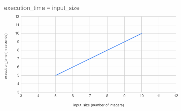
Consider the scenario where we are tasked with designing a program that operates on an array of 5 integers (the specifics of the program are irrelevant). Upon implementation, we conduct natural testing and observe that it takes 5 seconds to execute. Subsequently, we modify the input to utilize an array of 10 integers, run the program with these new arguments, and discern that it now takes 10 seconds to execute. From this observation, we can deduce that if we were to double the size of the inputs, the execution time also doubles: the relationship between execution time and inputs is linear.
Now, envision that we delve deeper into the literature and unearth an alternative approach for implementing this program. Equipped with this newfound method, we re-implement the previous algorithm, conduct another round of testing, and note that it now takes 0.5 seconds to execute with 5 integers and 1 second with 10 integers. From this, we can once again infer that if we were to double the size of the inputs, the execution time also doubles: the relationship between execution time and inputs remains linear.

Indeed, at first glance, the second method appears superior as it consumes less time with the same input. However, upon delving into additional research papers, we encounter a new algorithm. While it is somewhat more intricate, it takes 12 seconds to execute with an array of 5 integers and, surprisingly, also 12 seconds with an array of 10 integers. This method seems to be notably less favorable. Not only is it more challenging to implement, but it also requires more time to execute!
With a heightened awareness, we proceed to conduct experiments under real-world conditions using an array of 1000 integers. As anticipated, the first method takes 1000 seconds to execute, while the second method takes 100 seconds. However, quite surprisingly, the third algorithm once again takes only 12 seconds. Now, this third algorithm substantially outperforms the others!
There are several key insights to glean from this example.
- Firstly, the superiority of an algorithm can only be meaningfully studied and compared with asymptotic data, particularly as the input size becomes larger and larger. The third method mentioned earlier runs in constant time, exhibiting consistent performance regardless of input size, whereas the other two exhibit a time complexity proportional to the inputs.
- Secondly, even though the second algorithm may appear to run faster than the first one, this difference becomes less relevant for larger inputs. The crucial consideration is that its time complexity remains linear in relation to the size of the arguments passed.
Informally, we would say that the third algorithm executes in constant time or is an O(1) algorithm. On the other hand, the first and second algorithms execute in linear time and are O(n) algorithms.
In brief, big O notation allows developers and researchers to compare the efficiency of algorithms in a language-independent and platform-independent manner. It focuses on the high-level behavior of algorithms and is particularly useful when analyzing the scalability of algorithms for large input sizes. Keep in mind that while big O notation provides an upper bound, it doesn't capture constant factors, lower-order terms, or specific details of the implementation.
We did not delve into the gory details in this article, but big O notation can be made completely rigorous with a background in mathematics.
More information can be found here.
What are the Common Big O Notations?
Here are some common big O notations:
- O(1) - The time complexity is constant regardless of the input size. These algorithms are generally the best.
- O(logn) - The time complexity grows logarithmically with the input size. These algorithms are highly desired.
- O(n) - The time complexity is directly proportional to the input size.
- O(nlogn) - The time complexity is said to be linearithmic and is common in efficient sorting algorithms like merge sort and quicksort.
- O(n^2) - The time complexity is proportional to the square of the input size (quadratic). It is common in less efficient sorting algorithms.
- O(2^n) - The time complexity is exponential and the running time grows rapidly with the size of the input. These algorithms are generally useless on large inputs and must be avoided.
Enough Theory, Examples Please!
We will now provide a concrete illustration of the concepts discussed by comparing various algorithms for calculating the power of a real number. We will demonstrate that certain methods are significantly more efficient than others.
Given a real number x and an integer n, we aim to compute xn in an efficient manner. The code will be written in C#, but naturally, it is applicable to all other programming languages.
We will first define an IComputePower interface that all algorithms will implement.
public interface IComputePower
{
    double ComputePower(double real, int power);
}
Algorithm 1
The first algorithm is quite straightforward and does not need further explanation: we are simply applying the mathematical definition of a power.
public class LinearComputePower : IComputePower
{
    public double ComputePower(double real, int power)
    {
        var y = 1.0;
        for (var i = 0; i < power; i++)
        {
            y *= real;
        }

        return y;
    }
}
Analysis of the Algorithm
We denote T1(n) as the number of multiplications performed during the execution of the program. It is evident from the code that T1(n)=n (as n multiplications are performed in the for loop).
T1(n)=O(n)
Algorithm 2
This second algorithm is merely a recursive variant of the first algorithm.
public class LinearRecursiveComputePower : IComputePower
{
    public double ComputePower(double real, int power)
    {
        if (power == 0) return 1.0;
        return real * ComputePower(real, power-1);
    }
}
Analysis of the Algorithm
We denote T2(n) as the number of multiplications performed during the execution of the program. From the recursive form of the algorithm, we can express T2(n)=1+T2(n−1) for all n≥1, with T(0)=1. This forms an induction relation that mirrors the recursive aspect of the code. The resolution of this induction is quite straightforward, and T2(n)=n.
T2(n)=O(n)
Algorithm 3
The third algorithm we are examining is a more intricate method, based on the fact that if n is even, then xn=(x2)n/2, and if n is odd, then xn=x(x2)(n-1)/2. This provides a dichotomic method that can be recursively implemented.
public class DichotomyComputePower : IComputePower
{
    public double ComputePower(double real, int power)
    {
        if (power == 0) return 1.0;
        if (power == 1) return real;
        else
        {
            if (power % 2 == 0) return ComputePower(real*real, power/2);
            else return real * ComputePower(real*real, (power-1)/2);
        }
    }
}
We denote T3(n) as the number of multiplications performed during the execution of the program. We will not delve into the nitty-gritty details, but the time complexity can be precisely determined with some rather involved mathematics (see here for a complete proof). Here, we will content ourselves with the acknowledgment that T3(n)=O(log2n).
This algorithm appears to have a very desirable execution time and is superior to the others.
How to Verify Our Analyses ?
In this final section, we will attempt to demonstrate that our previous theoretical computations align with reality. To achieve this, we will intentionally introduce a Thread.Sleep instruction in our algorithm each time a multiplication is performed, and then we will execute the algorithms with various values of n.
For example, below is how our algorithm is modified with this instruction.
public class DichotomyComputePower : IComputePower
{
    public double ComputePower(double real, int power)
    {
        Thread.Sleep(1000);

        if (power == 0) return 1.0;
        if (power == 1) return real;
        else
        {
            if (power % 2 == 0) return ComputePower(real*real, power/2);
            else return real * ComputePower(real*real, (power-1)/2);
        }
    }
}
The main program will utilize a watcher to calculate the execution time.
public static void Main(string[] args)
{
    var watch = new Stopwatch();
    var x = 2; var n = ...;

    watch.Start();

    var computer = new DichotomyComputePower();
    var res = computer.ComputePower(x, n);

    watch.Stop();

    Console.WriteLine($"Time elapsed: {watch.ElapsedMilliseconds} ms, result: {res}");
}
Here are the results for various values of n.
It is evident that the third algorithm executes faster than the others. This confirms our earlier analyses.
Additional examples and the remainder of this article can be found here.
History
- 23rd November, 2023: Initial version
Nicolas is a software engineer who has worked across various types of companies and eventually found success in creating his startup. He is passionate about delving into the intricacies of software development, thoroughly enjoying solving challenging problems.


 General
  News
News  Suggestion
  Question
  Bug
Bug  Answer
  Joke
Joke  Praise
  Rant
Rant  Admin
Admin 


