Forecasting Stock Market Volatility with Kalman Filters

Introduction

There are many articles on how to predict the stock market's direction using machine learning models. But professionals like myself put just as much importance on assessing risk. Investors typically gauge risk using a metric called 'volatility,' which is the standard deviation of an investment's percentage changes in the past. This article shows you how to forecast volatility using one of my favourite machine learning models, the Kalman filter.

What is a Kalman Filter?

I won't regurgitate the precise mathematical structure of the Kalman filter here - you can find that elsewhere on the internet. Let me instead give a layperson's explanation of how the model works using a real-world usage example - tracking the position of a car using a GPS.

A travelling car will periodically receive its coordinates from satellites. The coordinates, however, are not precise - generally, GPS is only accurate to within 16 feet. When the car's navigation unit receives two different coordinates one after another, it has to figure out how much of the difference was caused by the car's movement and how much was due to measurement error. The navigation unit solves this problem using the Kalman filter.

Kalman filters pack the car's true coordinates and velocity in the state variable and assume that we can't observe that state directly. In the model, we specify how we expect the state to evolve. We can say, for example, that the car's next position will be the combination of its last position and velocity. We encapsulate such logic in the variable 'transition matrix.'

Kalman filters also allow the state to fluctuate randomly beyond that determined through the transition matrix. For example, we may model the car's next velocity as the last known velocity plus a random fluctuation. The car's driver wouldn't think of the velocity change as random since they usually cause it (e.g., by stepping on the brake). But the navigation unit doesn't understand the driver's intentions, so the velocity changes appear random, which is why the Kalman filter models it that way. We expect some bounds around the random fluctuations, though (we wouldn't expect velocity to go from 50km/h to 80km/h in a second), and we express those bounds statistically using the 'transition distribution.'

Once the car moves into a new state, the Kalman filter receives coordinates approximating its position. The 'observation matrix' describes what is observable - GPS can only observe the car's position, so the observation matrix disregards velocity. Observation entails random measurement errors, and the expected extent of those errors are expressed in the 'observation distribution''. You may wonder why we need separate distributions for transition and observation since they both add random noise to the data's journey from state to observation. The difference is that "noises" created during transition processes permanently alter the state, whereas those made during observation are transient.

I've thus far described how we go from a car's state to its observed values. To go from observed to state values, we must reverse-engineer this process. This is where we call on the magic of machine learning. Through Bayesian statistics, Kalman filters deduce the most likely state that would have produced the observations.

Stock market volatilities have similarities to the car-GPS example, making it amenable to Kalman filter modelling. On any given day, the market has a "true" volatility level around which observed volatility fluctuates. We assume this true volatility level changes randomly and that observed volatility centers around true volatility with random deviations.

Data Processing

Let's now get into the weeds of building a Kalman filter model. You can find the full Python code used in this article at https://github.com/moneygeek/kalman-filter-volatility-forecast. To keep this article from becoming a tome, I'll ignore some of the boilerplate and only explain those parts relevant to the Kalman filter.

We begin our programming journey by preparing the data. The code below downloads the historical price data of the SPDR S&P 500 ETF Trust, which we'll refer to by its ticker SPY. This instrument tracks the market-weighted average of the 500 largest stocks in the US, which serves as a good proxy for the entire US stock market. We only keep the final trading price of SPY on each day.

spy = yf.Ticker("SPY")
price_series = spy.history(period='max')['Close']

We next use the data we just downloaded to calculate the weekly volatility of SPY. We assign the trailing week's volatility to Fridays, the final trading day of each week.

volatility_series = price_series.pct_change().rolling('7D').std().dropna()
weekly_index = pd.date_range(volatility_series.index[0], 
                             volatility_series.index[-1], freq='W-FRI')
volatility_series = volatility_series.reindex(weekly_index, method='ffill')

A keen data scientist would notice a slight problem with this data construction. In normal weeks, our code calculates volatility using data from Mon to Fri. But if Friday is a holiday, the code pulls Thursday's data forward into Friday. Volatility on Thursdays incorporates data from the previous Friday to Thursday, but the previous week's volatility would likely calculate volatility using data from Monday to Friday. We thus use the previous week's Friday data twice - once for the last week's volatility and once again for the current week's. This problem is generally not a huge problem since few holidays fall on Fridays, but it's worth keeping in mind. I didn't correct the problem in this article to keep the code base small.

Let's now visualize volatility's data distribution. Visualization always helps us get a feel for the raw materials we're working with.

volatility_series.plot.hist(bins=30)
plt.show()<a href="https://drive.google.com/file/d/131xSp7rF0S7jlJWeh5uZ3x0zl1c6FMfd/
view?usp=drive_link" target="_blank"><img alt="" 
src="https://drive.google.com/file/d/131xSp7rF0S7jlJWeh5uZ3x0zl1c6FMfd/view?usp=drive_link"></a>

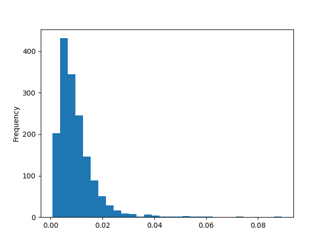
We notice a couple of things from the chart. The data is bounded below by 0, which makes sense since volatility can't be negative. We also notice that the data is skewed to the right. This skew would present problems down the road when we train Kalman filters - the model assumes that observed data will fluctuate by similar extents regardless of whether the deviations occur above or below true volatility. But the skew shows that fluctuations above true volatility can be much larger than fluctuations below. Thankfully, there's a simple remedy for this - we can take the natural log of the volatility data.

volatility_series = pd.Series(np.log(volatility_series.values), 
                    index=volatility_series.index).dropna()
volatility_series.plot.hist(bins=30)
plt.show()

That looks much better - the skew is gone, and the data distribution resembles a bell curve. A bell curve-shaped distribution is good for us since we can then use the Gaussian (a.k.a. 'Normal') distribution to model transition and observation distributions.

Next, we segment the training data from the test data. We set the training cutoff to be the beginning of 2020, which means we'll train our model using only data from before 2020 and test it with data after 2020. It would be as if we transported ourselves back to Jan 1, 2020, when we trained our model and assessed how it performed each week after that.

training_cutoff = datetime.datetime(2020, 1, 1, tzinfo=pytz.timezone('America/New_York'))
training_series = volatility_series.loc[volatility_series.index < training_cutoff]

Model Definition

Now that the data is ready, let's construct the Kalman filter model. I've chosen to build the model using the Pyro library. Pyro is not the simplest library you'll find - there are dedicated Kalman filter libraries that I could have used instead. But Pyro is much more versatile, enabling us to construct any other types of Bayesian machine learning models, so it's a better library to learn. It also allows me to highlight some details that may go hidden with other libraries.

The logic of the model is wrapped up in the following function definition. Parameter 'x' contains the sequence of SPY's volatilities. I'll explain warmup_periods later. We'll assume subsequent blocks of code will appear inside the forward method.

class VolatilityForecastModule(PyroModule):
   def forward(self, x: torch.Tensor, warmup_periods: int = 5):

The following code block sets up our expectations around the starting volatility value. It expresses our assumption that the true starting volatility is somewhere in the vicinity of the first observed volatility (i.e., x[0, 0]).

vol_loc = x[0, 0].unsqueeze(-1).unsqueeze(-1)
init_dist_scale = pyro.sample("init_dist_scale", dist.LogNormal(-2., 3.))
vol_scale = torch.tensor([[init_dist_scale]]).expand([1, 1, 1])

The proximity of the first observed volatility to the true volatility is expressed in the init_dist_scale parameter, with smaller numbers indicating they're closer. The precise estimate of init_dist_scale will be learned from the data when we train the model, but by sampling it from dist.LogNormal, we ensure that the value can't go negative. The vol_scale parameter represents the proximity between our current volatility estimate and the true volatility. This parameter starts off with the init_dist_scale value but will evolve later as we step through time increments.

The next code block defines the state transition behaviour.

transition_matrix = torch.tensor([[1.]])
transition_scale = pyro.sample("trans_scale", dist.LogNormal(-2., 3.))
transition_dist = dist.Normal(0., transition_scale.unsqueeze(-1)).to_event(1)

The transition matrix is [[1]], which means that, on average, we expect next week's true volatility to remain the same as this week's. Individual instances of volatility will deviate randomly from week to week, though, and the transition_scale parameter defines how much we expect the true volatility to fluctuate. Smaller values suggest minor changes in true volatilities from week to week. As with init_dist_scale, this parameter will be learned during training.

The next set of codes defines the relationship between true and observed volatilities.

observation_matrix = torch.tensor([[1.]])
observation_scale = pyro.sample("obs_scale", dist.LogNormal(-2., 3.))
observation_dist = dist.Normal(0., observation_scale.unsqueeze(-1)).to_event(1)

By setting the observation matrix to [[1.]], we say that observed volatilities will center around true volatilities with random deviations. The size of those deviations is represented by observation_scale, which will also be learned during training.

The next couple of lines use the variables we've seen thus far to forecast the true volatility of the subsequent week.

init_dist = dist.MultivariateNormal(vol_loc, vol_scale)
hmm = dist.GaussianHMM(
   init_dist,
   transition_matrix,
   transition_dist,
   observation_matrix,
   observation_dist,
   duration
)

init_dist defines the range where we're confident the true volatility resides, given the data we've seen thus far. hmm contains our forecast of where true volatility would go next. The forecast isn't a pinpoint estimate but a statistical distribution defining the range of possible values.

The following uses the subsequent week's data point to score how well its forecasts squared with the observation. You'll note that we finally use the warmup_periods variable defined in the forward method definition. Just as athletes need to warm up before performing at their full potential, Kalman filters must also digest a few data points before they start making their best forecasts. We, therefore, only grade models after they've warmed up.

next_x = x[0, t].unsqueeze(-1).unsqueeze(-1)
if t >= warmup_periods:
pyro.sample(f"obs_{t}", hmm, obs=next_x)

The above lines of code graded the model's performance, but it didn't let the model use the data to update its estimate of the true volatility. The next few lines of code do just that.

new_init_dist = hmm.filter(next_x)
vol_loc = new_init_dist.loc.detach()
vol_scale = new_init_dist.covariance_matrix.detach()

Finally, we store the new volatility estimate as the forecasted volatility for the period after next. In other words, if the previous input falls on week 1 and next_x comes on 2, the forecast is for week 3 made as of week 2. Such details are tedious but important to keep in mind.

forecasts.append((vol_loc).squeeze())

We run the code from init_dist = dist.MultivariateNormal(vol_loc, vol_scale) in a loop, stepping through time until we reach the final observed volatility.

Model Training

Having defined the model, let's now train it. The code in this section comes under the following function definition:

def train_model(training_series: pd.Series, epochs: int):

training_series contains the historical volatility data, and epochs is the number of times the data is fed to the model for it to learn. The following code creates the model object and the accompanying guide.

net = VolatilityForecastModule()
net = net.train()
guide = AutoDelta(net)

Pyro's guide is a complex concept, so let me oversimplify - it defines the shape of the trained parameters' statistical distributions. Recall that we want to find the values for three parameters - init_dist_scale, transition_scale, and observation_scale. Pyro is a powerful library. We could use it to find precise estimates for the parameters or, if we prefer, to find ranges of possible values instead. We don't go down that rabbit hole in this article. By using AutoDelta, we make the parameters take on specific numbers.

The next set of code executes the training.

optimizer = optim.Adam({
   'lr': 1e-3
})
svi = SVI(net, guide, optimizer, loss=TraceMeanField_ELBO())
for i in range(epochs):
elbo = svi.step(in_sample_data)

The optimizer governs the learning speed and style. The loss function TraceMeanField_ELBO is the grading system we use for scoring forecasts against data. elbo is the overall score. The absolute number of elbo doesn't matter, but we strive for lower numbers. The number should normally decrease with each epoch.

Training completes after the for loop exhausts the specified number of epochs. We can now generate predictions from the model using the predict function defined in the github repository's model/trainer.py. The code inside that function mostly consists of boilerplate, so I won't go through them here. Feel free to ask questions about specific lines of code that puzzle you.

Results

Let's see how well this model performs. But first, let's set some baseline expectations by showing you how well a naive forecast does. The naive forecast uses the previous week's observed volatility as the forecast for next week's volatility and is created using the following lines.

naive_results_df = volatility_series.to_frame('Actual').join(volatility_series.shift(1).to_frame('Forecast'))
naive_results_df = naive_results_df.loc[naive_results_df.index >= training_cutoff]

Notice that we only examine the period after the training cutoff date. We do this to facilitate like-for-like comparisons with our model's forecasts. Below are two charts that show the performance of the naive method.

The line chart (top) compares the forecasts and actuals across time. Unsurprisingly, they look almost identical since forecasts are just observations offset by a week. The scatter chart (bottom) gives us a better feel for its performance. The dots roughly line up diagonally from bottom left to top right, indicating that the naive method does a decent job of forecasting volatility. The R squared of the forecasts is 9.2%. Keep in mind that the analysis is for the logarithm of volatilities.

Let's see how our model fares in comparison. Below are the same charts that use model forecasts.

Notice how the forecasts mute some of the sharp ups and downs seen in the observed data. The scatter chart looks good, but it's hard to tell whether they're any better than the naive forecasts'. The R squared of the model forecasts is 28.5% - significantly better than the naive methods.

Let's now see how the forecasts look in the original volatility space. We can convert our logarithm data into original data by taking their exponents.

results_df = pd.DataFrame(np.exp(log_results_df.values), 
             index=log_results_df.index, columns=log_results_df.columns)

The following charts show how well the forecasts perform.

Intuitively, the forecasts look good. The R squared of these forecasts in the original space is 41.5%, even better than that witnessed in the log space. However, I caution against putting too much stock in this number. Because of the definition of the R squared, a few outlier data points in the original space can exert an inordinate influence on the R squared. If just one or two of the outlier data had not conformed well with the forecasts, the R squared would have been much lower in the original space. The log space R squared metric of 28.5% is the more accurate measure.

Accurate volatility forecasts are useful for many purposes, ranging from assessing the riskiness of a portfolio to informing on options strategies. I don't intend this code to be used for practical purposes, and the actual code I use is a fair bit more complicated. Instead, I hope this article has shown you the potential of using machine learning models such as the Kalman filter. That potential, as you can see, is pretty, pretty, good.

History

• 22^nd August, 2023: Initial version