Geospatial visualization using Python and freely available resources from Esri

One indicator of a region's growth is the number of permits issued for new construction. Exploring and analyzing permit activity can help regional planners ensure that development occurs in accordance to the area's long-term goals. One area that has recently experienced rapid growth is Montgomery County, Maryland, a suburban county near Washington, D.C. County planners want to observe spatial and temporal growth trends, find out why certain areas are growing faster than others, and communicate key information about the county's growth to the public.

In this example, we'll explore building permit data in Montgomery County, Maryland using freely available resources from Esri – the world’s leading location intelligence platform.

We will use the ArcGIS API for Python, a powerful and easy-to-use Python library used for managing, visualizing and analyzing data in a spatial context, alongside accessing content from ArcGIS Online – a SaaS based spatial analysis and mapping solution.

You can install it into your Conda environment using:

conda install -c esri arcgis

Once you have the ArcGIS API for Python ready to use, open a Jupyter notebook and import pandas and the ArcGIS API for Python.

from arcgis.gis import GIS
import pandas as pd
import seaborn as sns
import matplotlib.pyplot as plt
from arcgis.features import GeoAccessor, GeoSeriesAccessor

We will use the GIS module to connect into the freely available content from ArcGIS Online.

gis = GIS()

Search for the Commercial Permits since 2010 layer. We will specify the owner's name to get more specific results.

data = gis.content.search(
    'title: Commercial Permits since 2010 owner: rpeake_LearnGIS',
    'Feature layer')
data[0]

Get the first item from the results.

permits = data[0]

Geospatial data is often made up of multiple layers, using the ArcGIS API for Python we can use the layers property of this Feature Layer Collection which gives us a list of FeatureLayer objects within the collection. The permit layer is the first layer in this item.

permit_layer = permits.layers[0]

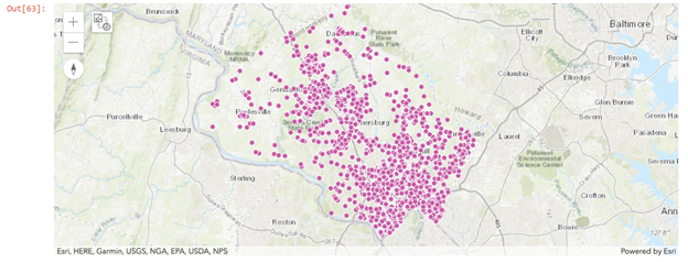
Next, we will visualize this layer on a map of Montgomery County, Maryland. To do this we first create a blank map and then add the layer to the map.

permit_map = gis.map('Montgomery County, Maryland’)
permit_map

permit_map.add_layer(permit_layer)

The map is fully interactive and can be panned, zoomed, and the points on the map can be clicked on to reveal a pop-up of with attributes about each point. However, rather than clicking on each point individually we can explore the data in a spatially enabled dataframe.

Data Exploration

Spatially enabled dataframes look and feel like pandas dataframes making them very easy to pick up and get started with.

First, let’s convert our spatial layer into a spatially enabled dataframe:

sdf = pd.DataFrame.spatial.from_layer(permit_layer)
sdf.head()

for col in sdf.columns:
    print(col)

We can also explore the data using charts:

plt.figure(figsize=(9,15))
ax=sns.countplot(y='Use_Code', data=sdf)

plt.axis('equal') 
permits_by_status.plot(kind='pie', legend=False, label='Permits by Status');

The pie chart above shows the four permit statuses, with the size of each status determined by the number of permits. The vast majority of permits are either Issued or Finaled. Finaled permits are issued permits that have also had the requisite inspections performed.

It is helpful to visualize the spatial distribution of permit attributes on a map. You'll change the map so that each permit's symbol represents its status.

permits_by_status_map = gis.map('Montgomery County, Maryland')
permits_by_status_map

sdf.spatial.plot(kind='map', map_widget=permits_by_status_map,
        renderer_type='u', # specify the unique value renderer using its notation 'u'
        col='Status')  # column to get unique values from

Visualize temporal and spatial trends

The data shows where permits have been opened and issued, but what do these permits say about when and where growth is happening in the county? The data also contains temporal attribute fields, such as Added_Date, which indicates when a permit was first added to the system. The field has several values that break down the data by year, month, and even hour.

We will split the Added_date to get year, month, week_of_day

sdf['datetime'] = pd.to_datetime(sdf['Added_Date'], unit='ms')
sdf['year'], sdf['month'], sdf['day_of_week'] = sdf.datetime.dt.year, sdf.datetime.dt.month, sdf.datetime.dt.dayofweek

sns.countplot(x="year", data=sdf);

The chart shows the number of permits issued each year since 2010. (The year 2017 has significantly fewer permits because the dataset only covers part of 2017.) You can compare the number of permits visually by the size of each bar. Although some fluctuation occurs from year to year, most years had similar permit activity.

Similarly, you can visualize it by month.

sns.countplot(x="month", data=sdf);

We can combine this information to visualize trends and patterns in permit issuance over time:

ddf['num'] = 1
ddf['num'].resample('M').sum().plot();

When we examine this chart, we see a huge spike in permit activity occurred in mid-2011.

What caused this spike? Is it an increase in overall permit activity, or is it mostly an increase in a certain type of permit? To better understand this outlier, we will plot the number of permits based on Use_Code to find out if any specific permit type one cased the spike.

fig = plt.figure(figsize=(15,5))
ax = fig.add_subplot(1, 1, 1)

ax.plot(ddf['num'].resample('M').sum(), 'k', label='Total permits')
for use_code in filtered_permits:
    x = ddf[ddf.Use_Code == use_code]['num'].resample('M').sum()
    ax.plot(x, label=use_code)
ax.legend();

Based on the legend, permit activity spiked in 2011 due to a sharp increase in the number of multifamily dwelling permits issued. This likely means that there was large residential growth in 2011.

The last question we will answer is where was the 2011 permit spike the densest? To do this we will use the temporal information we mined earlier and a hotspot map renderer.

hotspot_2011_map = gis.map('Germantown, Montgomery County, Maryland')
hotspot_2011_map

sdf[sdf.year==2011].spatial.plot(kind='map', map_widget=hotspot_2011_map,
        renderer_type='h',
        col='Status')  # column to get unique values from

For more information on spatial analysis and data science tools available in ArcGIS, visit Esri’s Spatial Analysis and Data Science page for details or join us for our upcoming free 6-week Spatial Data Science massive open online course (MOOC).

Also, if you are interested in kick-starting your own spatial analysis workflows with the ArcGIS API for Python, start for free with the ArcGIS for Developers Essentials Plan.