Boosting ODE simulations with Boost.odeint and Boost.SIMD

• Download odeint_simd.zip - 3.6 KB

Introduction

Ordinary Differential Equations appear in numerous applications and finding their solution is a fundamental problem in science and engineering. Often one has to rely on numerical methods to approximate such solutions as in the presence of nonlinearities, no analytic solution can be found. Being such a frequent problem, there exists a variety of libraries providing standard algorithms for numerically solving ODEs. Here, we will use the Boost.odeint library [1,2,3]. Boost.odeint is implemented in a generic way which makes it highly flexible. This flexibility will allow us to easily employ the SIMD capabilities of modern processors and reach significant speed-up of up to a factor three over standard implementations. To access this computational power we will make use of another tool: NT2's SIMD library [4,5,6] (proposed to become Boost.SIMD and from here on called Boost.SIMD). The generic design of odeint will allow us to use the SIMD data structures provided by Boost.SIMD in a transparent and simple manner. The programming effort from the standard implementation to SIMD ready code is virtually zero, which shows the importance and power of generic, well-designed libraries such as Boost.odeint and Boost.SIMD.

Ensembles of Ordinary Differential Equations

Ordinary Differential Equations (ODEs) are typically given in the following form:

d x(t) / d t = f( x(t) , t )

where x is said to be the state of the ODE (typically high-dimensional) and t is the dependent variable and the function f defines the ODE. One of the most prominent examples of ODEs are dynamical systems, where t represents time, x(t) is the trajectory resulting from the dynamics induced by f(x,t). Here, we will face the situation of having an ensemble of such dynamical systems all of which we want to integrate to obtain the trajectory for each of the systems. In this setup, all of the systems follow the same dynamical equation f(x,t), which will give us the possibility use SIMD instructions. A possible example for such a setup are Monte-Carlo simulations, but also parameter studies, where f(x,t) depends on some parameters which take different values for each realization of the ensemble.

In the performance tests below we will simulate an ensemble of Roessler systems. Each system of the ensemble has a three-dimensional state-space (x,y,z) and follows the following dynamical equations:

dx/dt = -y - z
dy/dt = x + ay
dz/dt = b + z(x-c)

with constants a, b and c which we set to some typical values: a=0.2, b=1.0, c=9.0. Our ensemble will consist of N such systems and we will use a different random initial condition for each system.

Implementation

We will start with a straight-forward implementation of the simulation based on Boost.odeint. From there we will add SIMD functionality using Boost.SIMD. We will see how little effort is required combining those two libraries and how much speed can be gained in our setup.

Simulating the Ensemble

With Boost.odeint, it is rather simple to implement the simulation outlined above. First, we have to choose the representation of the state of a single Roessler system. As the dimensionality of the problem is small, fixed and known at compile time, we choose a boost::array<double,3></double,3> for that. Then we provide the function f(x,t) in terms of a function object:

static const size_t dim = 3;  // roessler is 3D
typedef boost::array<double, dim> state_type;

//---------------------------------------------------------------------------
struct roessler_system {
    const double m_a, m_b, m_c;

    roessler_system(const double a, const double b, const double c)
        : m_a(a), m_b(b), m_c(c)
    {}

    void operator()(const state_type &x, state_type &dxdt, const double t) const
    {
        dxdt[0] = -1.0*x[1] - x[2];
        dxdt[1] = x[0] + m_a * x[1];
        dxdt[2] = m_b + x[2] * (x[0] - m_c);
    }
};

With this ingredients we can already simulate a single Roessler system. The following example iterates along a trajectory using the Runge-Kutta-4 algorithm with a step-size dt=0.1:

const int steps = 50;
const double dt = 0.01;
state_type x = {0.0, -1.0, 2.5};  // some "random" initial conditions
boost::numeric::odeint::runge_kutta4<state_type> stepper;
for( int step = 0; step<steps; ++step )
    stepper.do_step(roessler_system(0.2, 1.0, 9.0), x, step*dt, dt);

However, we want to simulate a whole ensemble of Roessler systems. One approach is to simulate the first system, then generate new initial conditions and simulate the next system and so on. But often you need to have the state of all systems available at each simulation step, e.g. for statistical analysis. Therefore, we introduce a vector that contains the states of all systems and subsequentally iterate over them at each step:

typedef std::vector<state_type> state_vec;
const int N = 1024*1024;  // number of systems in ensemble

state_vec state(N);

// generate random initial conditions...

boost::numeric::odeint::runge_kutta4<state_type> stepper;
roessler_system roessler(0.2, 1.0, 9.0);
double t = 0.0;
for( int step = 0; step < steps; ++step )
{
    for(size_t i = 0; i < N; ++i)
    {
        stepper.do_step(roessler, state[i], t, dt);
    }
    t += dt;
}

Note, that with state_vec state(N) a total of N*3*8 Bytes of continuous memory is allocated without any fragmentation that could introduce performance loss. Furthermore, odeint works only on one system at a time and uses boost::array for its internal temporary memory (defined by the template parameter of the stepper). Hence, no further memory allocations are performed in the code which allows for cache friendly code and excellent optimization possibilities for the compiler. Finally, the do_step method takes the state by reference and computes the result in-place, which means no unneccessary copy operations are performed.

The only thing omitted above is the initialization of the random initial conditions. We will use the <random> library introduced with C++11 to generate initial conditions and put them in our state_vec structure:

// random initial conditions
std::vector<double> x(N), y(N), z(N);
std::default_random_engine generator;
std::uniform_real_distribution<double> distribution_xy(-8.0, 8.0);
std::uniform_real_distribution<double> distribution_z(0.0, 20.0);
auto rand_xy = std::bind(distribution_xy, std::ref(generator));
auto rand_z = std::bind(distribution_z, std::ref(generator));
std::generate(x.begin(), x.end(), rand_xy);
std::generate(y.begin(), y.end(), rand_xy);
std::generate(z.begin(), z.end(), rand_z);

for(size_t i=0; i<n; ++i)
{
    state[i][0] = x[i];
    state[i][1] = y[i];
    state[i][2] = z[i];
}

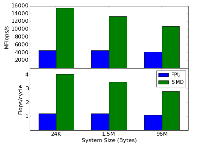
Now, we have all parts together and can run some performance tests of the simulation. All performance runs are done using the Intel Compiler v15.0 on an Intel Xeon E5-2690 CPU with 3.8 GHz (turbo mode). The graph below shows the performance of this implementation (blue bars) in MFlops/s (top graph) for several system sizes. As seen there, the performance is very good, reaching more than 1 Flops/cycle for all sizes. With utilizing only the FPU, one can reach not more than 1 Flops/cycle. The fact that our code performs even slightly better means that the Intel Compiler already uses some SIMD instruction via auto-vectorization. However, we can do much better in this example, as described below.

Using SIMD instructions

Starting from the code above we will now improve the performance using the Boost.SIMD library. With SIMD (Single Instruction Multiple Data), the processor is capable of performing a floating point operation on several values at a single clock cycle. Modern processor support the AVX instruction set that allows up to four additions and multiplications at once. In an optimal scenario, we can therefore hope to improve the performance by a factor of four on modern processors.

With help of Boost.SIMD, it is fairly simple to utilize this computational power of the CPU. Essentially, we only have to change the basic data type of the computations:

typedef boost::simd::pack<double> simd_pack;
typedef boost::array<simd_pack, dim> state_type;
typedef std::vector< state_type, boost::simd::allocator< state_type > > state_vec;

Instead of working with plain doubles, we use a boost::simd::pack. This is an abstraction of the SIMD registers provided by Boost.SIMD. Boost.SIMD already provides all basic operations on those SIMD packs, which means we do not have to change the roessler function at all! Note, that the SIMD instructions require aligned memory. To ensure that we get aligned memory in our state vector we use the simd::allocator from Boost.SIMD. All that is left to do is to take into account that we now already incorporate several systems at once in our SIMD pack and thus the state requries less entries. The size of the SIMD pack depends on the processor and can be accessed at compile time via simd_pack::static_size. With this, we can implement the simulation above using SIMD instructions:

static const size_t pack_size = simd_pack::static_size;
state_vec state(N/pack_size);

// Generate random initial conditions...

for(int step = 0; step < steps; step++)
{
    for(size_t i = 0; i < N/pack_size; ++i)
    {
        stepper.do_step(sys, state[i], t, dt);
    }
    t += dt;
}

That's really all! Boost.SIMD takes care of all the SIMD enhanced computations while Boost.odeint performs the ODE integration using the SIMD data type. The only place where we have to deal with the SIMD nature of the implementation directly is for generating the random initial conditions:

// random initial conditions for SIMD
std::vector<double> x(N), y(N), z(N);
std::default_random_engine generator;
std::uniform_real_distribution<double> distribution_xy(-8.0, 8.0);
std::uniform_real_distribution<double> distribution_z(0.0, 20.0);

auto rand_xy = std::bind(distribution_xy, std::ref(generator));
auto rand_z = std::bind(distribution_z, std::ref(generator));
std::generate(x.begin(), x.end(), rand_xy);
std::generate(y.begin(), y.end(), rand_xy);
std::generate(z.begin(), z.end(), rand_z);

state_vec state(N/pack_size);
for(size_t i=0; i<N/pack_size; ++i)
{
    for(size_t p=0; p<pack_size; ++p)
    {
        state[i][0][p] = x[i*pack_size+p];
        state[i][1][p] = y[i*pack_size+p];
        state[i][2][p] = z[i*pack_size+p];
    }
}

As you can see, we explicitly fill the SIMD types using the []-operator. As we only know at compile time how many SIMD register the target machine provides, we use a for-loop over the pack size to fill the registers. With this, we have completely transformed our ODE ensemble integration to utilize SIMD instructions. The graph above shows the performance of this implementation. And the result is very impressive. On the same Xeon E5-2690 CPU we reach almost 16 GFlops/s, or 4 Flops/cycle compared to the roughly 1.2 Flops/cycle of the standard implementation for small system sizes of about 32 KByte (1024 systems). Increasing the system size leads to clear performance decrease, because if the system gets to big it will not fit in the L1 cache and the CPU has wait for L2 (for very large systems finally also L3) cache loads from time to time which slows down the performance.

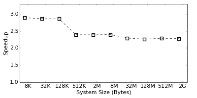
However, although the Flops/s is a good indicator for the efficiency of an implementation, the real performance can only be obtained by measuring the actual runtime of the simulation. The graph on the right shows the speedup of the SIMD implementation over the standard one in terms of the actual runtime improvement of the simulation. As seen, we reach a performance gain of a factor three for small, and a factor 2.4 for large systems. This numbers are slightly lower than the Flops/s improvement would suggest, but still quite impressive. Note, that the Flops are measured by the performance counters, which might not be 100% accurate. Hence, one should always rely on real runtime measurements to judge the performance of an implementation.

Summary and Conclusions

This article has shown how to utilize the full power of modern CPUs with C++ by means of combining Boost.odeint and Boost.SIMD. We were able to reach speedups of up to a factor three with almost no programming effort. This shows the importance and applicability of well-designed, generic C++ libraries such as Boost.odeint and Boost.SIMD. The examplary source code for an ensemble of Roessler systems can be easily generalized to other situations like parameter studies or ensembles of more complicated systems. Boost.SIMD provides an easy and nice abstraction of the SIMD capabilities of modern CPUs and should be considered for any performance-critical numerical algorithm. However, note that many algorithms are cache-bound rather than Flops-bound. In such situations one should focus on improving the cache usage before any SIMD tuning makes sense.

Acknowledgements

I thank Joel Falcou for pointing out the alignment requirement and giving further detailed feedback on the article. Furthermore, I thank Denis Demidov for proof reading the text.

This work was supported by the European Comission through the Marie Curie Initial Training Network Neural Engineering Transformative Technologies (NETT) under the project number 289146.

Ressources

Source Codes

The source codes for the simulations are available for download: odeint_simd.zip - 3.6 KB

Furthermore, the performance test has become part of Boost.odeint and can be found on Github.

References

[1] Karsten Ahnert and Mario Mulansky, odeint - Solving Ordinary Differential Equations in C++, AIP Conf. Proc. 1389 (ICNAAM 2011), pp. 1586-1589 (2011)

[2] odeint-v2 on Codeproject: http://www.codeproject.com/Articles/268589/odeint-v-Solving-ordinary-differential-equations

[3] odeint source code on Github: https://github.com/headmyshoulder/odeint-v2

[4] Pierre Estérie, Joel Falcou, Mathias Gaunard, Jean-Thierry Lapresté, Boost.SIMD: Generic Programming for portable Simdization, Proceedings of the 2014 Workshop on programming models for SIMD/Vector processing (2014)

[5] NT² SIMD library: http://www.numscale.com/boost-simd/

[6] NT² library on Github: https://github.com/MetaScale/nt2