In the previous blog posts, we covered some very interesting topics regarding Artificial Neural Networks (ANN). The basic structure of Artificial Neural Networks was presented, as well as some of the most commonly used activation functions. Nevertheless, we still haven’t mentioned the most important aspect of the Artificial Neural Networks – learning. The biggest power of these systems is that they can be familiarized with some kind of problem in the process of training and are later able to solve problems of the same class – just like humans do! Before we dive into that exciting topic, let’s have a quick recap of some of the most important components of artificial neural networks and its architecture.
The smallest and most important unit of the artificial neural network is the neuron. As in biological neural systems, these neurons are connected with each other and together, they have the great processing power. In general, ANNs try to replicate the behavior and processes of the real brain, and that is why their architecture is modeled based on biological observations. The same is with the artificial neuron. It’s structure is reminiscent of the structure of the real neuron.
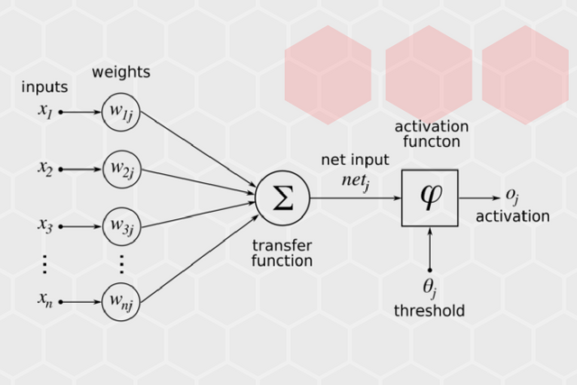
Every neuron has input connections and output connections. These connections simulate the behavior of the synapses in the brain. The same way that synapses in the brain transfer the signal from one neuron to another, connections pass information between artificial neurons. These connections have weights, meaning that value that is sent to every connection is multiplied by this factor. Again, this is inspired by brain synapses, and weights actually simulate the number of neurotransmitters that are passed over among biological neurons. So, if the connection is important, it will have a bigger weight value than those connections which are not important.
Since there could be numerous values getting into one of the neurons, every neuron has a so-called input function. Input values from all weighted connections are usually summarized, which is done by weighted sum function. This value is then passed to the activation function, whose job is to calculate whether some signal should be sent to the output of the neuron. You can read more about this in the previous article.
We can (and usually do) have multiple layers of neurons in each ANN. it looks something like this:

Learning
If we observe nature, we can see that systems that are able to learn are highly adaptable. In their quest to acquire knowledge, these systems use input from the outside world and modify information that they’ve already collected, or modify their internal structure. That is exactly what ANNs do. They adapt and modify their architecture in order to learn. To be more precise, the ANNs change weights of connections based on input and desired output.
“Why weights?”, one might ask. Well, if you look closer into the structure of the ANNs, there are a few components we could change inside of the ANN if we want to modify their architecture. For example, we could create new connections among neurons, or delete them, or add and delete neurons. We could even modify input function or activation function. As it turns out, changing weights is the most practical approach. Plus, most of the other cases could be covered by changing weights. Deleting a connection, for example, can be done by setting the weight to 0. And a neuron can be deleted if we set weights on all its connections to zero.
Training
In the first few sentences of this article, I mentioned one very, very important word for ANNs – training. This is a necessary process for every ANN, and it is a process in which the ANN gets familiar with the problem it needs to solve. In practice, we usually have some collected data based on which we need to create our predictions, or classification, or any other processing. This data is called training set. In fact, based on behavior during the training and the nature of training set, we have a few classes of learning:
-
Unsupervised learning – Training set contains only inputs. The network attempts to identify similar inputs and to put them into categories. This type of learning is biologically motivated but it is not suitable for all the problems.
-
Reinforcement learning – Training set contains inputs, but the network is also provided with additional pieces of information during the training. What happens is that once the network calculates the output for one of the inputs, we provide information that indicates whether the result was right or wrong and possibly, the nature of the mistake that the network made.
- Supervised learning – Training set contains inputs and desired outputs. This way, the network can check its calculated output the same as desired output and take appropriate actions based on that.
Supervised learning is most commonly used, so let’s dig a little deeper into this topic. Basically, we get a training set that contains a vector of input values and a vector of desired output values. Once the network calculates the output for one of the inputs, cost function calculates the error vector. This error indicates how close our guess is to the desired output. One of the most used cost functions is mean squared error function:
Here, x is the training input vector, y(x) is the generated output of the Artificial Neural Network and a is the desired output. Also, one can notice that this function is the function that depends on w and b, which represents weights and biases, respectively.
Now, this error is sent back to the neural network, and weights are modified accordingly. This process is called backpropagation. Backpropagation is an advanced mathematical algorithm, using which the Artificial Neural Network has the ability to adjust all weights at once. The important thing to remember here is that by using this algorithm, ANNs are able to modify weights in a fast and easy manner.
Gradient Descent
The entire point of training is to set the correct values to the weights, so we get the desired output in our neural network. This means that we are trying to make the value of our error vector as small as possible, i.e., to find a global minimum of the cost function. One way of solving this problem is to use calculus. We could compute derivatives and then use them to find places where is an extremum of the cost function. However, the cost function is not a function of one or a few variables; it is a function of all weights in the network, so these calculations will quickly grow into a monster. That is why we use the technique called gradient descent.
There is one useful analogy that describes this process quite well. Imagine that you had a ball inside a rounded valley like in the picture below. If you let the ball roll, it will go from one side of the valley to the other, until it gets to the bottom.
Essentially, we can look at this behavior like the ball is optimizing its position from left to right, and eventually, it comes to the bottom, i.e., the lowest point of the valley. The bottom, in this case, is the minimum of our error function. This is what gradient descent algorithm is doing. It starts from one position in which by calculating derivates and some second derivates of the cost function C, it gets the information about where “the ball” should roll. Every time we calculate derivates, we get information about the slope of the side of the valley at its current position. This is represented in the picture below with the blue line.
When the slope is negative (downward from left to right), the ball should move to the right, otherwise, it should move to the left. Be aware that the ball is just an analogy, and we are not trying to develop an accurate simulation of the laws of physics. We are trying to get to the minimum of the function using this alternative method since we already realized that using calculus is not optimal.
In a nutshell, the process goes like this:
- Put the training set in the Neural Networks and get the output.
- The output is compared with desired output and error is calculated using cost function.
- Based on the error value and used cost function, decision on how the weights should be changed is made in order to minimize the error value.
- The process is repeated until the error is minimal.
What I’ve just explained has one more name – Batch Gradient Descent. This is due to the fact that we put the entire training set in the network and then we modify the weights. The problem with this approach is that this way, we can hit a local minimum of the error function, but not the global one. The previous statement is one of the biggest problems in Neural Networks, and there are multiple ways to solve it.
However, the common way to avoid the trap of going to a local minimum is modifying weights after each processed input of the training set. When all inputs from a training set are processed, one epoch is done. It is necessary to do multiple epochs to get the best results. The explained process is called – Stochastical Gradient Descent. Also, by doing so, we are minimizing the possibility of another problem arising – overfitting. Overfitting is a situation in which neural networks perform well on the training set, but not on the real values later. This happens when the weights are set to solve only the specific problem we have in the training set.
Conclusion
Now, let’s sum this up in a few steps:
-
We randomly initialize weights in our neural network
- We send the first set of input values to the neural network and propagate values through it to get the output value.
- We compare output value to the expected output value and calculate the error using cost functions.
- We propagate the error back to the network and set the weights according to that information.
- Repeat steps from 2 to 4 for every input value we have in our training set.
- When the entire training set has been sent through the neural network, we have finished one epoch. After that, we repeat more epochs.
So, that is an oversimplified representation of how neural networks learn. What I haven’t mentioned is that in practice, the training set is separated into two parts and the second part of the training set is used to validate the work of the network.
Hopefully, this article will provide a good overview of the way neural networks learn. Since it is a complex topic, some things were left uncovered (backpropagation for example), which will be covered in the articles to come. It should be mentioned that I tried not to go too deep into the math, which leaves plenty of room for research.
Thanks for reading!


 General
  News
News  Suggestion
  Question
  Bug
Bug  Answer
  Joke
Joke  Praise
  Rant
Rant  Admin
Admin 


