Deep learning workloads have been growing at a rapid pace. Deep-learning-based algorithms process massive amounts of data to find patterns for image classification, object detection, time-series prediction, and much more. With the increase in data availability, the complexity of deep-learning models also increased. Models like ResNet* and Visual Geometry Group (VGG) have millions of parameters and perform on the order of billions of floating-point operations. Recent models, like Generative Pretrained Transformer 3 (GPT-3) and Bidirectional Encoder Representations from Transformers (BERT), have multi-billion to a trillion parameters. Therefore, training deep-learning models is a computationally expensive and time-consuming process. To reduce the time to a solution, apart from optimizing single- and multi-core performance, one might also consider scaling out to multiple nodes (for example, distributed training). This task can be achieved by splitting the model (model parallelism), splitting the data (data parallelism), or a combination of both schemes (hybrid parallelism).
This article focuses on tuning and scaling a deep-learning-based algorithm on a cluster of compute nodes. We illustrate using a semi-supervised generative adversarial network (S-GAN) to classify images. We demonstrate various tuning options in OpenMP*, TensorFlow*, and the Intel® MPI Library. On a single node, our optimizations achieve a 2x speedup. Scaling across an eight-node cluster achieves an overall speedup of 16x. Image throughput (images per second) for the Intel MPI Library was consistently better than the Open MPI* library by up to 27% on a single node and up to 18% on an eight-node cluster. Many of these performance gains were achieved without code modifications, indicating that these optimizations can be effectively applied to other applications.
S-GANs
Supervised learning requires large amounts of labeled data. Labeling and annotation must be done manually by human experts, so it is laborious and expensive. Semi-supervised learning is a technique where both labeled and unlabeled data are used to train the model. Usually, the number of labeled data points is significantly less than the unlabeled data points. Semi-supervised learning exploits patterns and trends in data for classification. Semi-supervised learning is a technique where both labeled and unlabeled data are used to train the model. Usually, the number of labeled data points is significantly less than the unlabeled data points. Semi-supervised learning exploits patterns and trends in data for classification.
S-GANs tackle the requirement for vast amounts of training data by generating data points using generative models. The generative adversarial network (GAN) is an architecture that uses large, unlabeled datasets to train an image generator model via an image discriminator model. GANs comprise two models: generative and discriminative. They are trained together in a zero-sum game. The generator’s job is to generate data similar to what's present in the dataset. The discriminator’s job is to identify the actual data among the generated data. S-GANs extend the GAN architecture by adding a supervised discriminator (classifier) to the classification task (Figure 1). This results in a classifier that generalizes well across unseen data.
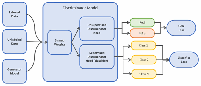
Figure 1. Architecture of S-GAN
Software and Hardware
Three Intel® oneAPI toolkits (v2021.1) were used for these experiments:
- Intel® oneAPI Base Toolkit
- Intel® oneAPI HPC Toolkit
- Intel® oneAPI AI Analytics Tool Kit
Intel® Distribution for Python* (v3.6), which uses Intel® oneAPI Math Kernel Library and Intel® oneAPI Data Analytics Library, was used to accelerate core Python numerical packages. The S-GAN model was implemented using Intel® Optimization for TensorFlow* (v1.15). Horovod* (v0.20.2) was used for distributed training. Horovod relies on MPI for internode communication, so the performance of two MPI libraries was compared: Intel MPI Library and Open MPI (v4.0.5). Intel® VTune™ Profiler was used to analyze performance. All tests were run on the Endeavor cluster from Intel using Intel® Xeon® Platinum 8260L processors, connected through the Intel® Omni-Path Fabric running at 100 Gbps (Figure 2).

Figure 2. Node composition ($ cpuinfo -g)
Tuning Methodology
It is good practice to measure baseline performance before optimizing an application. Profiling tools help identify areas for potential optimization, such as threading, vectorization, I/O, multi-node communications, and more. We used the Application Performance Snapshot in Intel VTune Profiler. The Application Performance Snapshot profile showed that far too many threads were being spawned by the application. Some threads came from OpenMP, while others came from the Eigen library that TensorFlow invokes. The number of OpenMP and Eigen threads exceeded the number of logical cores per node, resulting in resource oversubscription, which usually hurts performance.
Select the Optimal Number of Threads
The first step was to find the optimal number of threads. We tested different numbers of OpenMP threads by setting the OMP_NUM_THREADS environment variable on a single compute node using low-resolution images (256 x 256 pixels) and limiting the number of epochs (two) to save time. We found that 50 threads gave the best performance, with 19.67 images per second (Figure 3).
Figure 3. Find the optimal number of OpenMP threads
Next, we used the TensorFlow threading API to control the number of threads. The value of inter_op_parallelism_threads specifies the number of threads used by independent nonblocking operations, while the value of intra_op_parallelism_threads specifies the number of threads used for individual operations like matrix multiplication and reductions. Figure 4 shows the performance at different values of these two parameters. Dark green blocks indicate good performance, while dark red blocks indicate poor performance. White blocks indicate failed runs.
Figure 4. Find the optimal values of inter and intra_op_parallelism_threads.
For a single MPI rank per node, the optimal values of inter_op_parallelism_threads and intra_op_parallelism_threads were found to be 0 and 45, respectively, which corresponds to 12.34 images per second. This was lower than the value of 19.67 images per second achieved using OMP_NUM_THREADS (Figure 3), so we used this environment variable to control the number of threads instead of using the TensorFlow threading API.
Select the Optimal Number of MPI Ranks per Node
The application uses MPI and OpenMP hybrid parallelism, so it is important to find the best combination of OpenMP threads and MPI ranks per node. We repeated the test from Figure 3 (for example, 1 ≤ OMP_NUM_THREADS ≤ 96), but varied the number of MPI ranks per node (21 ≤ ppn ≤24, where ppn is the number of ranks per node, shown in Figure 5). The best performance (26.3 images per second) was achieved with eight MPI ranks and nine OpenMP threads on each node.
Figure 5. Find the best combination of OpenMP threads and MPI ranks in a single node
Overcome Memory Leakage
Low-resolution images were used for the experiments described so far. For higher-resolution images (1360 x 1360 pixels), the memory footprint of each worker process increased significantly, so running eight MPI ranks per node causes out-of-memory errors. It turned out that the memory footprint of a single rank was over 129 GB. With only about 200 GB of DRAM available on each node, it was only possible to launch a single rank per node, which would have been suboptimal for a dual-socket machine (because of non-uniform memory access [NUMA] issues). Running our application through the Memory Profiler for the Python utility revealed a memory leak. Around 56 GB of memory was not released during the forward pass of the model (Figure 6, top). This turned out to be a known bug (TensorFlow issue #33009 and Keras* issue #13118) in the Keras Model.predict method in TensorFlow. Based on recommendations from the TensorFlow community, Model.predict was replaced with Model.predict_on_batch, which lowered the overall per-process memory consumption (Figure 6, bottom). With the memory leak fixed, we were still limited to only two ranks per node for high-resolution images. We didn’t optimize the memory consumption further, although this might be possible.
Figure 6. A memory leak detected by the Memory Profiler
Set Other OpenMP* and Intel® MPI Library Environment Variables
The optimal settings of three other environment variables (KMP_BLOCKTIME, KMP_AFFINITY, and I_MPI_PIN_DOMAIN) were also explored. Based on previous performance recommendations, we ran the six experiments shown in Table 1. Note that the environmental variable settings in set #5 were also used in the other five sets. Set #3 gave the best training performance (Figure 7).
Table 1. Experimental settings for other OpenMP and Intel MPI Library environment variables
Figure 7. A performance comparison of the six experiments from Table 1
Choosing MPI Libraries
Next, we gathered the optimal settings from the previous tuning experiments and compared the performance of Intel MPI Library against Open MPI for the high-resolution images (1360 x 1360 pixels), with two MPI ranks per node and 33 OpenMP threads for a total of 100 epochs. The following Intel MPI Library command line was used:
$ OMP_NUM_THREADS=33 KMP_BLOCKTIME=1 I_MPI_PIN_DOMAIN=auto:compact \
    mpirun -n 2/4/8/16 -ppn 2 -f $HOSTFILE \
    python SGAN_pob.py --image_size 1360 --num_epochs 100 --save_checkpoints False
These roughly equivalent runtime settings were used for Open MPI*:
$ OMP_NUM_THREADS=33 KMP_BLOCKTIME=1 \
    mpirun - n 2/4/8/16 -hostfile $HOSTFILE - bind-to socket -map-by ppr:1:socket \
    --mca btl ^openib --mca pml ob1 --report-bindings - x LD_LIBRARY_PATH \
    python SGAN_pob.py --image_size 1360 --num_epochs 100 --save_checkpoints FALSE
Intel MPI Library outperformed Open MPI in single- and multi-node scenarios (Figure 8).
Figure 8. Performance comparison of Intel MPI Library and Open MPI
Although parallel scalability based on images per second appears linear, scaling based on time is sublinear, indicating application inefficiency. Further analysis revealed that the frequency of evaluations did not correctly scale according to the total number of nodes. As the number of nodes increased, so did the frequency of evaluations. Also, these evaluations were done by the MPI master rank, so all other ranks stalled until the master rank finished the evaluation. We fixed this issue by performing the evaluation step every 15 training iterations, regardless of the number of nodes (Figures 9 and 10). This modification did not affect model accuracy.
Figure 9. Fraction of total time spent on training and evaluation before optimization (left) and after optimization (right)
Figure 10. Multi-node performance with linear time scaling
Conclusions
In this article, we presented an incremental optimization approach to achieve better S-GAN training performance. Both runtime and source code-based optimizations were performed to resolve memory issues, scaling issues, and single-node performance inefficiencies. Horovod was used to implement distributed training of the S-GAN model on a multi-node cluster. Two MPI libraries (Intel MPI Library and Open MPI) were compared.
Figure 11. Final speedup obtained with Intel MPI Library
Figure 11 summarizes the performance gains from our optimization effort. The single-node optimizations achieved a 2x speedup, while multi-node optimizations resulted with a further 8x speedup, bringing overall time-to-solution down by a factor of 16, with no loss in model accuracy.
This member has not yet provided a Biography. Assume it's interesting and varied, and probably something to do with programming.
This member has not yet provided a Biography. Assume it's interesting and varied, and probably something to do with programming.


