Construction of Sparse Matrices for Finite Elements with TBB Containers and OpenMP

Introduction

The Finite Element Method (FEM) was conceived as an engineering tool for calculating forces in trusses. It allowed engineers to "see" forces that are invisible to the naked eye. It was quickly realized that aside from analyzing static force distributions, FEM can be applied in various areas of physics - Fluid Mechanics, Heat Transfer, Electromagnetism. In general, FEM is a way of "solving" differential equations by converting them to something that a computer "understands" - floating-point arithmetic.

While there are various types of FEM, many of them come down to crunching a linear system of equations in the form

where \(\mathbf{A}\) is a sparse matrix.

Libraries that solve such equations already exist - MKL, LAPACK, cuSPARSE - to name a few. FEM codes prepare the matrix \(\mathbf{A}\) and the right-hand side \(\mathbf{b}\) and let a solver do its magic. But how exactly is the sparse matrix prepared? Is there a way to optimize this process?

During my several years in academia, I wrote an algorithm for the assembly of sparse matrices. This data structure is unlike any other. It is a non-standard mapping with specific properties. Most attempts to go with the "standard" hash sets and red-black trees go terribly wrong.

This article will discuss the possible pitfalls with the assembly of sparse linear systems. It may be helpful to researchers who develop custom FEM implementations.

A Simple Example

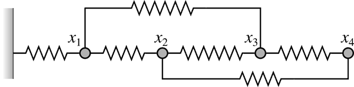
Consider a mass-spring system, where each spring has its unique stiffness constant \(k_n\) and a rest length \(d_n\). A spring \(n\) that connects nodes \(i\) and \(j\) exerts the following force onto node \(i\).

For every force acting on node \(i\), there is a force with an opposite sign acting on the incident node \(j\):

We are looking for the nodal displacements at equilibrium - when all forces from the springs add up to zero:

A linear system of equations arises:

where \(\mathbf{x}=[x_1,x_2,...,x_N]^T\) is the nodal positions vector, \(\mathbf{A}\) is a matrix of nodal interactions, and \(\mathbf{b}\) is the right-hand side of the linear system. The latter is non-zero because the initial spring lengths \(d_n\) contribute constant terms.

The length of \(\mathbf{x}\) will be denoted as N, and the size of matrix \(\mathbf{A}\) is NxN.

For each spring that connects the nodes \(i\) and \(j\), there are non-zero entries \(e_{ii},e_{ij},e_{ji},e_{jj}\) in matrix \(\mathbf{A}\). Aside from these elements, the matrix is mostly filled with zeros - it is sparse.

This article will discuss the ways of preparing and storing sparse matrices for FEM applications.

COO List - Super Easy

Most solver libraries accept sparse matrices in the so-called Coordinate List (COO) format, which represents the non-zero entries as (row, column, value) tuples. Row and column are encoded as integers, whereas value entries have the floating-point type.

To create such a list of tuples, one would iterate over all springs and append the corresponding entries to the list.

// make a stretchy list
std::vector<std::tuple<int,int,double>> COO_list;

// append values from each finite element
for(const auto &spring : springs)
{
  COO_list.insert(A.end(),spring.Entries_A());
}

This can be accomplished in parallel with OpenMP and TBB containers:

// a container that will survive simultaneous insertions
tbb::concurrent_vector<std::tuple<int,int,double>> COO_list;

// go parallel!
#pragma omp parallel for
for(unsigned i=0;i<springs.size();i++)
{
  const Spring &spring = springs[i];
  A.push_back(spring.Aii());
  A.push_back(spring.Aij());
  A.push_back(spring.Aji());
  A.push_back(spring.Ajj());
}

There are a few problems with this approach.

1. Since all threads append the entries simultaneously to the same container, there are frequent race conditions. Concurrent containers work best when the race conditions are infrequent.
2. Some (row,column) pairs may appear more than once. The solver will subsequently add them together, but they take more memory than needed.
3. For solvers, COO is not a convenient format, so they will spend time converting it to a more suitable representation.

Despite the obvious limitations, this assembly method is probably the best tradeoff between code complexity and performance. It is definitely a good option, especially for research codes that do not push the RAM/CPU limits.

Flawed Options that are Worse than COO

In systems with more than a million variables, the assembly step may take a significant amount of time. Unlike the one-dimensional spring model, which creates four entries per spring, some FEM elements may create much larger entries. For example, a cohesive zone element may connect two quads, i.e., affect eight nodes. Additionally, each node may have three degrees of freedom (xyz), making each sub-entry of size 24x24, giving a total of 576 double-precision values. Storing all entries in a list may affect performance and consume more memory than needed.

Since each row of the matrix contains at least one non-zero entry, the matrix is dense in its rows. One may try to store it as a vector of vectors of pairs:

std::vector<std::vector<std::pair<int,double>>> crazy_vector;

Some sparse matrix libraries use this approach because it allows the insertion of new non-zero entries by dynamically resizing the arrays. This storage format also facilitates iterating over row entries, which simplifies matrix multiplication algorithms.

The problem is that none of these benefits speed up the assembly process. Re-allocation of the vectors leads to memory fragmentation and overall performance loss, while insertion operations on vectors are super slow.

Addressing the Problem

Sparse matrix libraries provide on-the-fly resizing, but for most FEM applications, this is not needed. Since we know which elements connect to which nodes, we can infer the locations of non-zero entries upfront before their values are computed.

This brings us to the Compressed Sparse Row (CSR) format, which is a native internal representation in many solvers. Submitting this format to a solver will not trigger a conversion step. Unlike other representations, it is not suitable for dynamic resizing, but it is efficient for storage and access.

In CSR, non-zero entries are stored sequentially in a single allocated block. Before that block is allocated, the "sparsity structure" is created, i.e., the list of non-zero entries should be known. For the mass-spring example, the code would look something like this:

// STRUCTURE CREATION STAGE

// will store (i,j)-indices of non-zero entries
std::vector<std::pair<int,int>> s;

// iterate over the list of springs, and "mark" which matrix entries are used
for(const auto &spring : springs)
{
  s.emplace_back(spring.i, spring.j);
  s.emplace_back(spring.j, spring.i);
}

// add diagonal entries
for(int i=0;i<N;i++) structure.emplace_back(i,i);

// sort the resulting list -
// the consecutive elements of a row will reside next to each other
std::sort(s.begin(),s.end());

// remove duplicates
s.resize(std::distance(s.begin(),std::unique(s.begin(), s.end())));

// NNZ is the number of non-zero entries
unsigned NNZ = s.size();

// prepare a block of memory for non-zero values
std::vector<double> values;
values.resize(NNZ);

// READY TO COMPUTE THE MATRIX!

The resulting structure vector s contains one (i,j)-entry for each non-zero element of the sparse matrix. The size of s is the number of non-zero elements, denoted as NNZ.

This approach looks very similar to the first attempt with the COO list. We are simply creating the COO list without the actual values. The algorithm marks which (i,j) cells are in use, removes the duplicates and prepares a single memory block for the values.

But now the values are in a separate list!

Why are two lists better than one? Well, the assembly stage can now be truly parallel. Race conditions will occur when two springs write into the same (i,j)-cell. Such a situation, while not impossible, is very unlikely. So the assembly stage has improved. A typical implementation would look like this:

// ASSEMBLY STAGE

// reset the matrix to zero
std::fill(values.begin(), values.end(), 0);

// additively populate the entries of the matrix from each spring
#pragma omp parallel for
for(unsigned i=0;i<springs.size();i++)
{
  const Spring &spring = springs[i];
#pragma omp atomic
  values[get_offset(spring.i, spring.i)] += spring.Aii();
#pragma omp atomic
  values[get_offset(spring.i, spring.j)] += spring.Aij();
#pragma omp atomic
  values[get_offset(spring.j, spring.i)] += spring.Aji();
#pragma omp atomic
  values[get_offset(spring.j, spring.j)] += spring.Ajj();
}

Mappings, Mappings...

We now need a mapping function get_offset(int i, int j) that points to where each (i,j)-entry is stored. A naive solution would be to use std::map or std::unordered_map, but let's consider the downsides.

1. These data structures allocate memory dynamically every time they are prepared.
2. The insertion complexity is O(log(NNZ)), so for several million NNZs there will be a perceivable performance hit.
3. Sorting (or maintaining the sorted order) of the (i,j)-list is computationally expensive.

Final Solution

Let's use the fact that our sparse matrix is dense in terms of rows. We know that each row contains at least one non-zero entry, and the number of rows N is known upfront. Thus, (i,j)-pairs can be represented as a vector of vectors (again).

// expected number of non-zero entries per row
constexpr unsigned nCon = 8;

// each row will store indices of the connected neighbors
std::vector<std::unique_ptr<tbb::concurrent_vector<unsigned>>> rows;

// preallocate upfront
// avoid copying the whole "vector of vectors" by using pointers
if(rows.size()<N)
{
  rows.reserve(N);
  while(rows.size()<N)
    rows.push_back(std::make_unique<tbb::concurrent_vector<unsigned>>(nCon*2));
}

We are back to where we started, but not quite. This time the situation is different. We are not dynamically allocating the whole matrix but only the structure arrays. In fact, we avoid unnecessary reallocations altogether.

The maximal number of entries per row is more or less known upfront - it depends on a particular FEM algorithm and the mesh type. Still, it is usually constant within a given application. For example, in 2D meshes with triangular elements, each node is typically surrounded by 6-7 triangles. Storing this upper bound in nCon constant ensures that the row vectors will not exceed their initial capacity. Additionally, this whole memory structure can be reused on subsequent computation steps, and allocation only happens once.

Finally, since the TBB concurrent vectors are used, the structure can be populated in parallel. I have not compared the sequential and parallel algorithms, but the parallel is probably faster for extra-large meshes, while the sequential is optimal for smaller geometries. For the sequential algorithm, one could use Boost's small vector boost::container::small_vector<unsigned,nCon*2>.

Let's see how the non-zero elements are marked.

// STRUCTURE CREATION STAGE - each spring "marks" its non-zero matrix entries
#pragma omp parallel for
for(unsigned k=0;k<springs.size();k++)
{
  const Spring &spring = springs[k];
  rows[spring.i]->push_back(j);
  rows[spring.j]->push_back(i);
}

Instead of sorting one ginormous array of (i,j)-indices, we now sort many small arrays in parallel! The duplicate (i,j)-entries are removed as before. Finally, we count the total number of nonzero elements NNZ, which will be needed in the next step.

// SORT EACH ROW SEPARATELY AND REMOVE THE DUPLICATES; COUNT NNZ

// counter for the total number of non-zero entries
unsigned NNZ = 0;

// process rows in parallel
#pragma omp parallel for reduction(+:NNZ)
for(unsigned i=0;i<N;i++)
{
  tbb::concurrent_vector<unsigned> &rn = *rows[i];

  // add the diagonal entry
  rn.push_back(i);

  // sort the column indices (j-entries)
  std::sort(rn.begin(),rn.end());

  // remove the duplicates
  rn.resize(std::distance(rn.begin(),std::unique(rn.begin(),rn.end())));

  // count the non-zero entries
  NNZ += rn.size();
}

We now proceed with creating the structure arrays COL_INDEX and ROW_INDEX, which are a part of the CSR representation and passed to the solver. They also allow an O(1) lookup in the (i,j)->(offset) mapping. The size of COL_INDEX is NNZ, and the size of ROW_INDEX is N+1. We store both arrays as std::vector<int> and resize as needed. To populate them, we iterate over the sorted (i,j)-pairs and enumerate the entries sequentially.

// PREPARE CSR STRUCTURE ARRAYS
std::vector<int> COL_INDEX, ROW_INDEX;

// resize as needed
COL_INDEX.resize(NNZ);
ROW_INDEX.resize(N+1);
ROW_INDEX[N] = NNZ;

// enumerate the sorted indices to populate COL_INDEX and ROW_INDEX
unsigned count = 0;
for(unsigned row=0;row<N;row++)
{
  ROW_INDEX[row] = count;
  tbb::concurrent_vector<unsigned> &rn = *rows[row];
  for(unsigned const &local_column : rn)
  {
    COL_INDEX[count] = local_column;
    count++;
  }
}

Last Piece of the Puzzle

At the assembly stage, the matrix entries are additively written into the values array. For each (i,j)-entry, there is an offset to a memory location. It is important to infer these offsets efficiently because this operation repeats numerous times. In the earlier versions, I tried various approaches, starting from a straightforward std::map<std::pair<int,int>,int>, then evolving into per-row maps, and even a separate vector of vectors. But is there a better way?

There is an elegant way to use COL_INDEX and ROW_INDEX. The latter already stores the offsets to the first non-zero element in each row, ROW_INDEX[i]. We just need to find the column-index that matches j.

We iterate through a portion of COL_INDEX between &COL_INDEX[ROW_INDEX[i]] and &COL_INDEX[ROW_INDEX[i+1]], and find the value that matches j.

// for a given (i,j)-entry, return an offset in the array of values
unsigned get_offset(int row, int column)
{
  // where the row begins
  int col_offset_begin = ROW_INDEX[row];

  // where the row ends
  int col_offset_end = ROW_INDEX[row+1];

  // subrange in COL_INDEX that stores j-indices for a given row
  int *start_pt = &COL_INDEX[col_offset_begin];
  int *end_pt = &COL_INDEX[col_offset_end];

  // run a binary search on COL_INDEX to find our "column"
  auto it = std::lower_bound(start_pt, end_pt, column);
  return std::distance(start_pt,it)+col_offset_begin;
}

I am not exactly sure whether the binary search std::lower_bound or a regular search std::find is faster in this case. Depending on a particular FEM setup, rows may have very few entries, so a direct linear search may perform better. Either way, this is an elegant solution with constant time lookup.

Conclusion

There are numerous varieties of Finite Element Methods. Students and researchers are constantly inventing new modifications. Not all FEM codes use sparse matrices - some can do without them. This article does not claim to suggest the most optimal algorithm - it's and algorithm that works, and there is room for optimizations.

In my Ph.D. and Postdoc research, I wrote various FEM codes - materials with cohesive zones, shell and plate elements, 2D Neo-Hookean materials, among other things. Some used linear solvers, others used quadratic optimizers. My focus was more on FEM formulations rather than the implementation of the matrix math. Indeed, some competitive programmers would quickly come up with an optimal assembly procedure, but for me, this code was slowly evolving into its current shape over many years. A working project the uses this algorithm can be found here. Please do not hesitate to leave a comment, especially to suggest improvements. This algorithm may have practical value for other FEM researchers, and that's the motivation for this article!