A description and comparison of logistic regression, back propagation and support vector machine processing the Iris data set
Introduction
In machine learning, quite often, the task is to try to create an algorithm that is capable of giving a certain conclusion according to some input data and this conclusion shall be based on some earlier gathered data. A simple sample for such a task could be to find the minimum required effort for students to learn for an exam. If we have, for instance, the data of 7 students: Learning hours and success at the exam (a popular example :-))
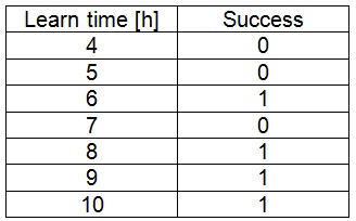
A computer program should compute the shortest required learning time to succeed at the exam.
OK. That’s just a sample. I don’t want to bother with such simple things (anyhow: the solution should be around 6.9 hours).
I think for such tasks, there are three important algorithms that might be interesting to be known:
- Logistic regression
- Back propagation
- Support vector machines
and a fourth one, which is the base for two of the above ones.
- Gradient descend
All four algorithms do the same: answering questions like the above one. But their way of doing this is different and the answers they can provide are different as well. Some comparison is quite interesting.
The procedure to apply them is for all the same: Use an existing data set with some input features x1, x2, x3,… and a property y that should be guessed later on, and train a software to recognize the input features and guess the property correct. The training is done in an iterative process for all.
I implemented the three algorithms and processed the Iris data set with them for comparison.
Iris Data Set
The Iris data set is a popular data set to work on such issues. It is a very nice data set containing characteristic data of 150 Iris flowers: The size of its flowers.
It contains the following information in one row:
- sepal length in cm
- sepal width in cm
- petal length in cm
- petal width in cm
- class:
- Iris Setosa
- Iris Versicolour
- Iris Virginica
The idea is to guess the correct flower class according to the measurement of its flower.
For each algorithm, I implemented a training application and a test application. I split the 150 samples into 135 samples for training and 5 of each flower for testing. I know, only 15 samples for testing is not too much. But I think it’s just enough for the understanding :-)
But first, a small introduction to the algorithms:
Gradient Descend
Gradient descend is an algorithm that tries to approximate a function like:

onto a given set of data samples (x1, x2, x3…,y). Depending on the required output, the approximating function can be linear or polynomial or just a differentiable function. With this approximation, it can guess the property y of another data sample (x1, x2, x3…,?) of which the property y is not known. It is in this form mainly used to guess a real value as the property of the data sample. For instance, if we have some characteristic data of wine like alcoholic content, sugar content, acidity… and the property is a quality rating between 1 and 10. That would be solved be the gradient descend algorithm.
The approximating function f(x) should match the property y as good as possible. Therefore f(x) is brought into relation to the property by calculating the deviation of all training samples like:
This deviation is usually called the cost of the optimisation and it is a validation of the quality of the approximation. The smaller it is, the better is the approximation. This cost should be minimized and this is done by the gradient descent algorithm. Therefore, the gradient of the cost function is built and starting from a random point the algorithm runs down this gradient as long as it is not 0. The movement is done by a relatively small step size: The so called learning rate. This learning rate affects the convergence behaviour quite strong. If it is too big, the algorithm starts to oscillate and never finds the minimum. If it is too small, the algorithm will fall asleep and never reaches the minimum. Usually, it should be smaller the more data samples have to be processed.
(For a detailed description of the gradient descend algorithm, see http://www.mosismath.com/AI/GradientDescend.html.)
Logistic Regression
Logistic regression is an algorithm that is based on the Gradient Descend algorithm but its purpose is to approximate a function with digital output 0 or 1. Its output is a probability. Similar to Gradient Descend, it tries to approximate a function like:
But this function is fed into a so called trigger function which is usually the Sigmoid function.
This g(x) is used for the optimisation and should match the property y (which has a value 0 or 1) as good as possible. Now g(x) is brought into relation to the property by calculating the deviation of all training samples like:
The sigmoid function is 0 for big negative input values and approaches 1 for big positive input values.
Shape of the sigmoid function
That converts the output of the approximation into a probability between 0 and 1 which is <0.5 for y = 0 and >0.5 for y = 1. The Logistic Regression is used to guess digital properties (see http://www.mosismath.com/AI/LogisticRegression.html for a detailed description).
Processing the Iris Data Set with Logistic Regression
To process the Iris data set with logistic regression, first the task must be split in three parts:
The algorithm shall first check whether the data sample belongs to the class Iris Versicolor. If not, it shall check if the sample belongs to the class Iris Setosa and if this is also not the case, it shall finally check for the class Iris Virginica. That looks like:
That means we have to train 3 settings and get 3 parameter sets that can easily be copied from the training application into the test application. OK, the last step could be skipped but I think it is a nice net like that. :-)
An important point to note: The last knot has an output “No Iris Virginica”. This will never be active with these data. The algorithm can only distinguish the trained classes and as there is no class included which is none of the three flowers, the algorithm will never classify a sample as none of these three classes.
We first have to determine the approximating function to be used. As the measurements of the flowers fit to one particular flower class only within a certain range, the approximating function should be a polynomial of second degree for each feature like:
For the training, I prepared three data sets. One for the first class, one for the second and one for last class.
With these, I got the following parameters:
Iris Versicolor
With a cost of 0.0166 after 132772 iterations.
Iris Setosa
With a cost of 0.00046 after 5148 iterations
Iris Virginica
With a cost of 0.0116 after 8653 iterations
With these parameters implemented in the test application, all 15 test data samples are recognised correct with a mean probability of 91% and the cost of each training result is relatively small that’s quite cool.
Back Propagation
Logistic regression handles approximating functions with one linear or polynomial function and one trigger function. Back propagation treats a complex net of functions consisting of more than one trigger function and its input function which is usually the sum of all knots of the preceding layer multiplied each by a linear factor: A neural net. This net contains several layers: An input layer that takes the features of one data sample, one or more hidden layers that contain the approximation functions including their triggers and an output layer that transmits the result to the outer world. That makes a net of several knots where usually, there is a connection from each knot of one layer to each knot of the next layer and each connection symbolizes an input function for the succeeding knot an each knot, except the input knots, contains a trigger function.
Neural net with 2 hidden layers
Back Propagation is mainly used to approximate more complex functions with digital output. For each data sample, it runs first from left to right in the net and computes the output value for one sample. Then it runs from right to left and computes the correction of the parameters in the net for this one sample according to the deviation of its output. These two procedures are called forward propagation and back propagation and they are carried out for each data sample and at the end of such a loop, the parameters are corrected by the mean of all these corrections and the loop is repeated until the minimum deviation is reached.
(For a detailed description of the algorithm, see http://www.mosismath.com/AI/BackPropagation.html.)
Processing the Iris Data Set with Back Propagation
To process the Iris data set, I set up the neural net like:
With four inputs, one hidden layer and two outputs that give out the number of the flower class in binary form like:
Iris-setosa => output 1 = 0 ; output 2 = 0

Iris-versicolor => output 1 = 1 ; output 2 = 0

Iris-virginica => output 1 = 1 ; output 2 = 1
Basically, it would be possible to use only one output and to train 3 different settings. But the back propagation algorithm works better, the more outputs are used.
With this setting, I can process the entire data set at once. I just have to set the two outputs for the training accordingly.
With this setting, the backpropagation algorithm computes the values:
with:
Cost = 0.0145854 after a fixed number of 60000 iterations.
I hard coded them in the test application and all 15 test samples were recognised correct with a mean probability of 98%. That’s quite a bit better than the logistic regression algorithm did.
Support Vector Machine
The support vector machine is different from the above algorithms. It does not approximate a function but classify data. In a very simple sample: If there is a data set containing the features x1, x2 and the property y which is a value 1 of -1, the support vector machine tries to lay a line between the data samples with y = 1 and the ones with y = -1 like:
On this sample image, the red points are the ones with y = 1 and the blue points the ones with y = -1. The black line is the separating line. Additionally, there are two grey margin lines. These 3 lines should be laid the way that no points lay between the margin lines and the distance between the margin lines is as big as possible (the length of the vector u-v). OK, this is a very simple and uncommon example. But the support vector machine algorithm is capable of solving much more complicate tasks. In multi-dimensional cases, it lays not a line but a hyperplane between the samples.
Principally, the support vector machine computes a vector W and an offset b that yields for each data sample:
A constant value b adds to the property y multiplied by the dot product of W and x, where x is a vector of all input features.
Now there are usually more complex situations than displayed in the picture above. The input features consist of more dimensions and the separation cannot be done by a straight line. The support vector machine algorithm can handle multi-dimensional cases and to virtually bend the separating line or hyperplane, the so called Kernel trick is used.
(For a detailed description of the algorithm, see http://www.mosismath.com/AI/SMO.html.)
There are several different approaches to solving the optimisation problem of a support vector machine. I implemented the sequential minimal optimization algorithm by John C. Platt. That’s one of the simplest approaches and it works fine.
Processing the Iris Data Set With the Support Vector Machine
As the support vector machine classifies the data in two classes in one setting, the task must be split in two. First, I want to classify whether the data sample is of the class Iris Setosa or not. If not, I want to classify whether it is of the class Iris Versicolor or not and if it is not, it is of the class Iris Virginica. Therefore, I had to prepare two data sets for training. The support vector machine needs the property y as value 1 or -1. So for the first training data set, I have to set the property = 1 for all data samples of class Iris-Setosa and = -1 for all others and second data set contains only data samples of Iris Versicolor and Iris Virginica and all samples of class Iris Versicolor get the property = 1 and all the rest 0 -1.
As there can result quite a many support vectors as output of the training, I could not just copy paste them from the training application to the test application. So they are transferred by a .Json file. The first classification yields 10 support vectors after 6 iterations and the second one yields 38 support vectors after 15 iterations.
With these parameters, all test samples were all recognised correct. There is no probability available here. But a measure for the quality of the separation is the value of the f(x). This should not be between 1 and -1. That’s the target. But that might not be reachable in most cases. So it is OK if the values are not too close to 0. The test application finds three values around -0.6. That’s quite good. :-)
Conclusion
The result of all three algorithms looks quite simple and straight forward. But that might mislead a little. All three algorithms approach their result in an iterative process starting at a particular point. They are searching for the minimum of a function. The complexity of this function is not the same for all and they do not just find the best result at once. The setting of start parameters and the fine tuning of iteration parameters is for all of them not too simple.
The gradient descend algorithm uses a more or less simple approximating function. But some say that the gradient descend algorithm converges not too fast and tends to oscillate. I say that can be avoided quite a bit by implementing it a little differently. According to the literature, the offset value of the approximating function is updated in the same loop as all the other values are updated. That influences one another and makes the algorithm prone to oscillations. If the offset is treated separately, the algorithm converges way faster and seems to oscillate much less (see http://www.mosismath.com/AI/LinregIterative.html). That makes the gradient descend algorithm quite an interesting approach for many problems.
The backpropagation algorithm is quite fancy in machine learning. But it consists usually of more than one knot containing a trigger function in the form of the sigmoid function. Each such knot brings more complexity and local minimums into the approximating function. That means the more knots the neural net contains, the more likely the algorithm gets hanging at a local minimum instead of finding the global minimum we are looking for. That makes it quit difficult to set the best starting point for the iteration and to find the global minimum. That’s the main reason why the input function of the triggers is usually the sum of just a linear multiplication of the preceding knots and not a polynomial. That would bring even more complexity into the system. Backpropagation is a very strong algorithm but it is not too easy to be run. It requires quite a lot of trial and error for starting points and setting up of trigger functions to find the searched solution.
The support vector machine algorithm is quite a sophisticated and smart algorithm. But its success depends strongly on the correct selection and setting of the used Kernel function. If the algorithm is not well fine-tuned, it can output a big amount of supporting vectors. So it’s always worthwhile spending some time to find the best setting for it. With the Iris data, it converged very fast. That’s not always the case. It can take quite some time to complete the calculations if there are many data samples and many input features combined with a complicate Kernel function.
Compared one to each other, the gradient descend algorithm is surely the simplest solution (I like that :-)). But not every data set can be approximated by a mathematical function as the gradient descend algorithm (or the backpropagation) does it. And not every data set can be classified by a support vector machine. So there might always be some trial and error and fine tuning required.
All three algorithms cannot just be fed with some data, be run and yield a useful result. They all require some attention by the user. But that’s exactly what makes the field of artificial intelligence fascinating. Before artificial intelligence can start, there will always be some human intelligence that is required. :-)
This article has been translated to Chinese and posted on the Chinese Software developer Network. See
https://blog.csdn.net/mzl87/article/details/107126598#%E6%A2%AF%E5%BA%A6%E4%B8%8B%E9%99%8D
I appreciate that and say thank you very much to the kind Chinese fellow who did that :-)
For further reading about maximum log likelihood
http://www.mosismath.com/AI/MaxLoglikelihood.html
or
http://www.mosismath.com/AI/BackPropagationMaxLog.html
could be interesting :-)
History
- 1st May, 2020: Initial version


 General
  News
News  Suggestion
  Question
  Bug
Bug  Answer
  Joke
Joke  Praise
  Rant
Rant  Admin
Admin 


