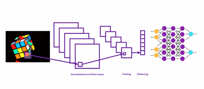
Have you ever wondered how Snapchat detects faces? How do self-driving cars know where a road is? You are right, they are using a special kind of neural network used for computer vision – Convolutional Neural Networks. In the previous article, we had a chance to examine how they work. We covered layers of these networks and their functionalities. Basically, additional layers of Convolutional Neural Networks preprocess image in the format that standard neural networks can work with. The first step in doing so is detecting certain features or attributes on the input image. This is done by convolutional layer.
This layer uses filters to detect low-level features, like edges and curves, as well as higher levels features, like a face or a hand. Than Convolutional Neural Network uses additional layers to remove linearity from the image, something that could cause overfitting. When linearity is removed, additional layers for compressing the image and flattening the data are used. Finally, this information is passed into a neural network, called Fully-Connected Layer in the world of Convolutional Neural Networks. The goal of this article is to show you how to implement all these concepts, so more details about these layers.
Before we wander off into the problem we are solving and the code itself, make sure to setup your environment. As in all previous articles from this series, I will be using Python 3.6. Also, I am using Anaconda and Spyder, but you can use any IDE that you prefer. However, the important thing to do is to install Tensorflow and Keras.
MNIST Dataset
So, in this article, we will teach our network how to recognize digits in the image. For this, we will use another famous dataset – MNIST Dataset. Extending its predecessor NIST, this dataset has a training set of 60,000 samples and testing set of 10,000 images of handwritten digits. All digits have been size-normalized and centered. Size of the images is also fixed, so preprocessing image data is minimized. This is why this dataset is so popular. It is considered to be a “Hello World” example in the world of Convolutional Neural Networks.

MNIST Dataset samples
Also, using Convolutional Neural Networks, we can get almost human results. Currently, the record is held by the Parallel Computing Center (Khmelnitskiy, Ukraine). They used an ensemble of only 5 convolutional neural networks and got the error rate of 0.21 percent. Pretty cool, isn’t it?
Importing Libraries and Data
Like in previous articles in this series, we will first import all necessary libraries. Some of these will be familiar, but some of them we will explain a bit further.
import numpy as np
from matplotlib import pyplot as plt
from keras.utils.np_utils import to_categorical
from keras.models import Sequential
from keras.layers.core import Dense, Dropout, Flatten
from keras.layers import Conv2D, MaxPooling2D
As you can see, we will be using numpy, the library that we already used in previous examples for operations on multi-dimensional arrays and matrices. Also, you can see that we are using some features from Keras Libraries that we already used in this article, but also a couple of new ones. Sequential and Dense are used for creating the model and standard layers, i.e., fully-connected layer.
Also, we can see some new classes we use from Keras. Conv2D is a class that we will use to create a convolutional layer. MaxPooling2D is a class used for pooling layer, and Flatten class is used for flattening level. We use to_categorical from Keras utils as well. This class is used to convert a vector (integers) to a binary class matrix, i.e., it is used for one-hot encoding. Finally, notice that we will use matplotlib for displaying the results.
After we imported all necessary libraries and classes, we need to take care of the data. Lucky for us, Keras provided MNIST dataset so we don’t need to download it. As mentioned, all these images are already partially preprocessed. This means that they are having same size and digits displayed on them are properly positioned. So, let’s import this dataset and prepare data for our model:
from keras.datasets import mnist

(X_train, y_train), (X_test, y_test) = mnist.load_data()

rows, cols = X_train[0].shape[0], X_train[0].shape[1]
X_train = X_train.reshape(X_train.shape[0], rows, cols, 1)
X_test = X_test.reshape(X_test.shape[0], rows, cols, 1)

X_train = X_train.astype('float32')/255
X_test = X_test.astype('float32')/255

num_of_classes = len(set(y_train))
y_train = to_categorical(y_train, num_of_classes)
y_test = to_categorical(y_test, num_of_classes)
As you can see, we imported MNIST dataset from the Keras datasets. Then we loaded data in train and test matrices. After that, we got the dimensions of images using shape property and reshaped input data so it represents one channel input images. Basically, we are using just one channel of this image, not the regular three (RGB). This is done to simplify this implementation. Then we normalized the data in the input matrixes. In the end, we encoded the output matrixes using to_categorical.
Model Creation
Now, when data is prepared, we can proceed to the fun stuff – the creation of the model:
model = Sequential()

model.add(Conv2D(32, kernel_size=(3, 3), activation='rectifier', input_shape=(rows, cols, 1)))
model.add(Conv2D(64, kernel_size=(3, 3), activation='rectifier'))
model.add(Conv2D(128, kernel_size=(3, 3), activation='rectifier'))

model.add(Dropout(0.5))

model.add(MaxPooling2D(pool_size = (2, 2)))

model.add(Flatten())

model.add(Dense(128, activation='relu'))
model.add(Dropout(0.5))
model.add(Dense(num_of_classes, activation='softmax'))

model.compile(loss= 'categorical_crossentropy', optimizer='adam', metrics=['accuracy'])
We used Sequential for this, of course, and started off by adding Convolutional Layers using Conv2D class. As you can see, there are few parameters this class is using, so let’s explore them. The first parameter is defining a number of filters that will be used, i.e., number of features that will be detected. It is a common procedure to start from 32 and then go to bigger number of features from that moment on. That is exactly what we are doing, in the first convolutional layer, we are detecting 32 features, in the second 64 and in the third and final 128 features. Size of the filters that will be used is defined using next parameter – kernel_size, and we have chosen 3 by 3 filters.
For the activation function, we are using rectifier function. This way, we are adding non-linearity level automatically with every Convolutional layer. Another way to achieve this, and a bit more advanced, is by using LeakyReLU form keras.layers.advanced_activations. This is not like standard rectifier function, but instead of squashing all values that are below a certain value to 0, it has a slight negative slope. If you decide to use this, beware that you have to use linear activation in Conv2D. Here is an example of how that would look like:
from keras.layers.advanced_activations import LeakyReLU

model.add(Conv2D(32, kernel_size=(3, 3), activation='linear',input_shape=(rows, cols, 1)))
model.add(LeakyReLU(alpha=0.1))
We digressed for a bit. Let’s get back to Conv2D and its parameters. Another very important parameter is input_shape. Using this parameter, we are defining dimensions of our input image. As mentioned, we are only using one channel, that is why the final dimension our input_shape is 1. Other dimensions we picked up from an input image.
Also, we added other layers to our model too. Dropout layer is helping us with overfitting, and after that, we added pooling layer by using MaxPooling2D class. This layer is apparently using the max-pool algorithm, and size of the pooling filter is 2 by 2. Pooling layer is followed by Flattening layer, which is followed by Fully-connected layer. For the final Fully-Connected layer, we added the neural network with two layers, for which we used Dense class. In the end, we compiled our model, and we used Adam optimizer.
Training
Very well, our data is pre-processed and our model created. Let’s merge them together, and train our model. For this, we are using, already familiar, function fit. We pass the input matrices and define batch_size and number of epochs. Another thing we are doing is defining validation_split. This parameter is used to define which fraction of testing data is going to be used as validation data.
Basically, the model will set aside part of training data, but it will use it to evaluate the loss and other model metrics at the end of each epoch. This is not the same as testing data because we are using it after every epoch.
model.fit(X_train, y_train, batch_size=128, epochs=20, verbose=1, validation_split=0.2)

score = model.evaluate(X_test, y_test, verbose=0)

print('Accuracy:', score[1])
After that, our model is trained and ready. We are using evaluate method and pass testing set to it. Here, we will get the accuracy of our Convolutional Neural Network.
Predictions
One more thing we could do is to gather predictions of our network on the test dataset. This way, we can compare predicted results with actual ones. For this, we will use predict method. Using this method, we can also make predictions on a single input.
predictions = model.predict(X_test)
Results
Let’s use these predictions we just gathered for the final touch of our implementation. We are going to display predicted digit, with the actual one. And we will display the image for which we made the prediction. Basically, we will make nice visual representation for our implementation, after all, we are processing images here.
plt.figure(figsize=(15, 15))
for i in range(10):
    ax = plt.subplot(2, 10, i + 1)
    plt.imshow(X_test[i, :, :, 0], cmap='gray')
    plt.title("Digit: {}\nPredicted:    {}".format(np.argmax(y_test[i]), np.argmax(predictions[i])))
    plt.axis('off')
plt.show()
Here, we used pyplot to display ten images with actual result and our predictions. And this is how it looks like when we run our implementation:
We have run twenty epochs and got the accuracy – 99.39%. Not bad at all. There is always room for improvement, of course.
Conclusion
Convolutional Neural Networks are one very interesting sub-field and one of the most influential innovations in the field of computer vision. Here, you could see how to implement one simple version of these networks and how to use it for detecting digits on MNIST dataset.
Thanks for reading!


 General
  News
News  Suggestion
  Question
  Bug
Bug  Answer
  Joke
Joke  Praise
  Rant
Rant  Admin
Admin 


